A hierarchical model for hockey scoring

Background

They say one of the first things you should do when writing is establish credibility. I like to zag where other people zig, so here’s an unfortunate fact: I’ve done a terrible job of closely following sports outside of baseball since working in the industry. However, I try to pay attention to major storylines, and one that’s been interesting to me this year is the Bruins 18-3 start to the season.

This is particularly interesting to me because individual hockey outcomes are very random. On any given day, the worst team could beat the best and nobody would bat an eye. Looking at the FiveThirtyEight game predictions, most win probabilities are between 40-60% and the max is around 70%. That’s why seasons are long: to wash the variance out over a large sample size and allow us to get a better understanding of the true talent. So for a team to come out 18-3, there’s probably a good amount of luck folding into that, and I was curious if a quick model could give an understanding of just how lucky they’ve gotten.

Methodology

The model of choice to model NHL team strength is one that I’ve found particularly clean, originally by Baio and Blangiardo for football (soccer), and has been applied to several different goal-scoring in fixed-time sports. Goal scoring, \(y = (y_{g0}, y_{g1})\), is modeled as a Poisson process:

for game \(g\), with \(j = {0, 1}\) an indicator variable for home ice. In their paper the rate parameter \(\theta_{gj}\) is given by the following:

Here \(h\) is the home ice advantage, \(a\) is the “attack strength,” \(d\) is the “defense strength,” and \(h\) and \(v\) denote “home” or “visitor” respectively. Last, \(\alpha\) is a flat intercept. In words: the home scoring rate is proportional to the attack skill of the home team, minus the defense of the away team, plus home ice advantage. The away scoring rate is the opposite, with no advantage.

Last, these parameters must have priors. This is approached using a hierarchical approach in which the team attack and defense parameters are themselves drawn from a shared distribution. By taking a hierarchical approach, we can use the knowledge that while each offense can be strong or weak, offense is a similar concept so we can share information between the population, by drawing their parameter values from the same distribution (and similarly for defenses). This causes what’s known as Bayesian shrinkage bringing what may normally be extreme values in a non-hierarchical model closer to the population mean.

The priors are here, using a non-centered parameterization to help sampling run computationally smoother.

For team attack strength \(a_i\) (in this case \(\mu\) denoting the mean of the population attack strength). Similarly, for defense:

for team \(i\). And finally,

These Poisson processes are fit simultaneously. This is done using pymc, the full code can be seen in Appendix 1. I adapt this model using data from the 2022-2023 hockey season thus far (330 games). The observed values that the model is fit on are the end of regulation scores, in order to maintain consistent time lengths over which the Poisson process is observed.

While I maintain the approach of the original paper, here forward I substitute the language of “attack strength” for goal-creation strength and “defense strength” for goal-suppression strength in order to articulate that the defensive measures wrap up both goalie and defense effects into one latent parameter.

Results

Posterior Latent Parameter Values

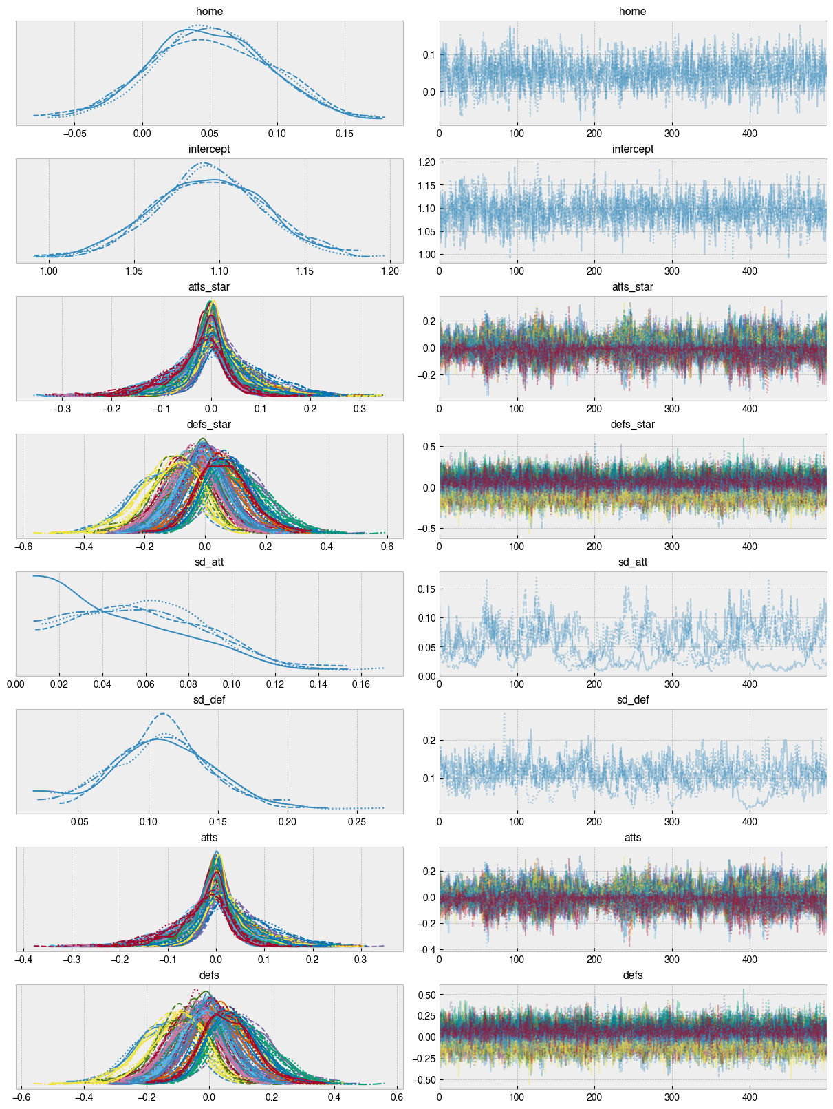
This model fits well (trace plots in Appendix 2). The parameters most of interest here are the latent goal creation and suppression strengths for each team, so without further ado,

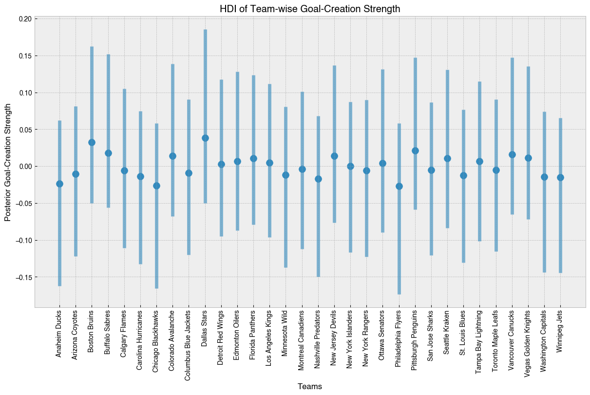
We can see that given just about 20 games per team, there’s not a lot of daylight in goal creation ability yet. The Bruins are near the top, but Dallas takes the number one spot in terms of the median value. Of course, this being a Bayesian model, we can see that uncertainty still dominates here.

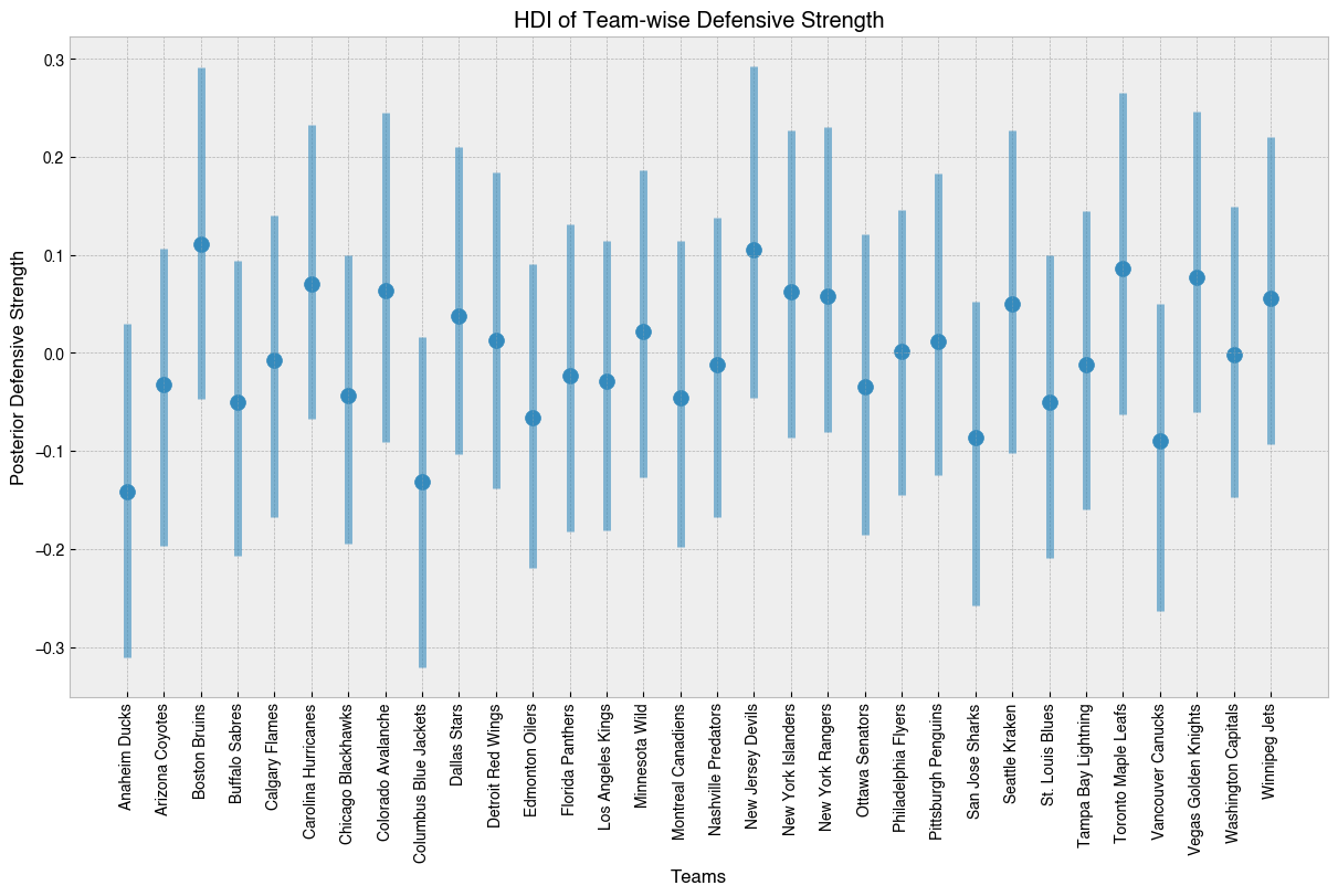
Similar goes for goal suppression ability, however there’s a bit more separation here. We can see that the Bruins and Devils top the league in goal suppression ability, while Columbus and Anaheim are notably lagging.

We can plot the medians of our posterior distributions for our parameters on a 2D plane to understand overall skill.

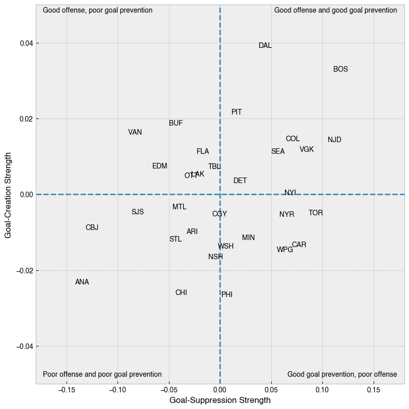
Here we can see that due to having the best score differential (+37), the model believes Boston does in fact sit at the top-right corner of this plane, and the wins seem to be pretty well balanced between goal creation and suppression. On the flip side, Anaheim’s -36 goal differential lands them on the opposite corner. Vancouver, in the top left corner, has scored the 9th most points, but given up the 5th most, giving high scoring play that still leaves them 23rd overall. Calgary takes the honor of being closest to league average over both metrics.

Posterior Predictive Distribution

Last we want to take a look at the posterior predictive distribution. Using the sampled values for parameters, if we reran the matches, what would we expect scoring and win totals to look like.

This does create a problem though: by construction this model does not forbid ties, the two Poisson processes can yield the same number of goals. However to estimate win totals, we will have to decide those ties.

This was done in a bit of an ad-hoc way. For each simulated season, I took the number of decided wins and number of decided losses for a given team, these would be proportional to their goal creation and goal suppression ability, so it made sense to use. Of the decisions, I created a “win-rate,” \(p_{i}\) given by decided wins divided by total decided matches for each team. In each given matchup, if the Poisson processes yielded a tie, I rolled a Bernoulli trial, with success probability equal to the harmonic mean of \(p_{ih}\) and \((1-p_{iv})\). If the trial is successful, the home team wins the tie, otherwise the away team does.

After this, we can rerun the season to this point, given our modeled team-level run creation and run suppression ability. Of our 2000 simulated seasons to this point, here’s the number of wins the bruins had in each:

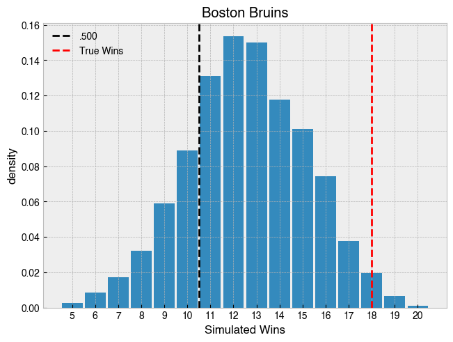
The most likely outcome for the Bruins given their above average goal creation and suppression ability is 12 wins. They’ve blown that out of the water with 18, which they achieve that many or greater in just 2.7% of seasons simulated.

This can be repeated for every team:

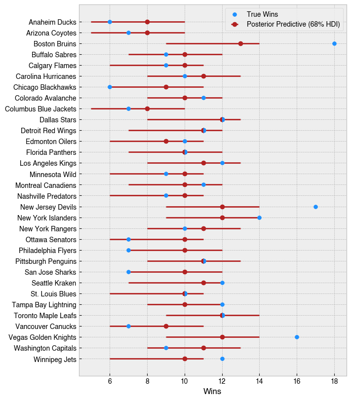
Here, the posterior median wins and 68% highest density interval (HDI) is shown. The Bruins have the highest median wins, but only edging out the Devils, Islanders, Maple Leafs, and Golden Knights by one win. The max wins covered by their HDI matches those teams as well.

Summary

In high variance sports, typically I think of individual outcomes as biased coin flips: good teams will win slightly more often, bad teams will lose slightly more often, and long seasons allow us to see the degree of that bias. The output of this model depicts a picture that is much closer to that mental model, compared to what an 18-3 team would otherwise evoke. The most common alternate reality created by this model has the Bruins with just 12 wins, indicating it seems they’ve gotten fairly lucky so far. At the risk of stating the obvious, I would not expect them to continue winning at this clip, but specifically the model suggests expecting closer to a 57% win percentage (12 wins in 21 games) based on the derived parameters.

That being said, this model is built on a slightly shaky foundation, and there is room for improvement. The first major issue is that the only data input into this model is scoring in regulation, in an attempt to stay true to the Baio and Blangiardo model, as well as to fulfill the requirement of Poisson distributions to be count-based data. However, there is randomness in actual goal scoring, and something like expected goals (xG), conditional things like shot location, defender proximity, etc. have proven to be more predictive of future performance, and taking such an approach would likely yield better estimates.

Secondarily, latent goal creating and goal suppressing parameters are very broad concepts. Sweeping goal tending and defense into one parameter is definitely not the best possible approach here, and the easiest gain might be to model goal tending itself - possibly by using shots on goal as a Poisson process, and playing a similar game where the rate is lowered by a latent skill parameter of the opposing goalie.

All in all, this study allowed me to employ a model which I’ve found quite clean on an interesting use-case, the Bruins hot start, giving insights into goal creation and goal suppression ability league-wide so far this year.

Code to replicate this study can be found on GitHub, and data is pulled from the Hockey-Reference Schedule and Results.

Citations

Gianluca Baio and Marta Blangiardo. Bayesian hierarchical model for the prediction of football results. Journal of Applied Statistics, 37(2):253–264, 2010.

Appendices

1.

with pm.Model(coords=coords) as model:

    # constant data
    home_team = pm.ConstantData("home_team", home_idx, dims="match")
    away_team = pm.ConstantData("away_team", away_idx, dims="match")

    home_score = pm.MutableData("home_score", df_f.regulation_home_score, dims="match")
    away_score = pm.MutableData("away_score", df_f.regulation_away_score, dims="match")


    # global model parameters
    home = pm.Normal("home", mu=0, sigma=0.2)
    intercept = pm.Normal("intercept", mu=0, sigma=2)

    # attacks
    sd_att = pm.HalfCauchy("sd_att", 0.2)
    atts_star = pm.Normal("atts_star", mu=0, sigma=sd_att, dims="team")

    # defs
    sd_def = pm.HalfCauchy("sd_def", 0.2)
    defs_star = pm.Normal("defs_star", mu=0, sigma=sd_def, dims="team")

    # team-specific model parameters
    atts = pm.Deterministic("atts", atts_star - at.mean(atts_star), dims="team")
    defs = pm.Deterministic("defs", defs_star - at.mean(defs_star), dims="team")
    home_theta = at.exp(intercept + home + atts[home_idx] - defs[away_idx])
    away_theta = at.exp(intercept + atts[away_idx] - defs[home_idx])

    # likelihood of observed data
    home_points = pm.Poisson(
        "home_points",
        mu=home_theta,
        observed=home_score,
        dims=("match"),
    )
    away_points = pm.Poisson(
        "away_points",
        mu=away_theta,
        observed=away_score,
        dims=("match"),
    )

    trace = pm.sample(500, tune=500, cores=4)

2.

• 2023 1
• 2022 2
• 2021 1
• 2020 10
• 2019 8
• 2018 3
• 2017 1