Classifying MLB Hit Outcomes - Part 4: Application and Reflection

Over the last 3 posts, I’ve shown the construction of a model to predict hit outcomes based on kinematics such as the launch angle, exit velocity, and spray angle, as well as additional properties such as sprint speed and park factors. In this post, I’ll look at an application of it, and do some final reflections on the utility of this model.

Application - Model-Based wOBA

A common stat to evaluate offensive production is Weighted On Base Average (wOBA). This stat tries to encapsulate the idea that various offensive actions are worth different values, and weight them proportionally to the observed “run value” of that hit. For a trivial example, envision a case where there’s only a baserunner on second. A walk cannot move that baserunner, where a single can advance them, so a single ought to be weighted worth more than a walk. The weights for those actions are derived from data, looking at how often they translate to actual run production, using a method known as linear weights.

To calculate wOBA, multiply each offensive result that advances baserunners (BB, HBP, 1B, 2B, 3B, HR) by its relative weight, and sum. Then, divide that value by all possible opportunities. Explicitly,

where variables preceded by “n” indicate “number of” (e.g. n1B = number of singles), and variables with “w” indicate a weight. The linear weights vary year-to-year based on run environment.

The problem with wOBA is that it is calculated based on outcomes, but there’s a level of uncertainty in outcomes - variance due to things like defense or weather. This works as a description of events that happened, but not for an understanding of underlying skill. By focusing on wOBA, we do what Annie Duke calls “resulting” in her book Thinking in Bets - fixating solely on the outcome, neglecting the quality of inputs. In other words, if contact would result in a single 90% of the time, but the outcome is one of the unlucky 10% that is an out, we reduce our understanding of underlying quality hit by counting it as an out.

This is a perfect opportunity to utilize the hit classification model. The model outputs how likely it thinks a given hit by a player is to end up being a single, double, triple, home run, or out. For example, it might say a line drive has a 30% chance of an out, 40% chance of a single, 20% chance of a double, 10% chance at a triple, and isn’t hit hard enough for a HR, so 0% chance. We can put these likelihoods into the wOBA equation in order to get a wOBA based on the probability the model assigns to all possible outcomes, rather than that of only the result. To do so, in the equation above, the counts of each hit type need to be replaced by the sum of probabilities for the respective hit type (e.g. n1B is replaced by the sum of each hit’s probability to be a single).

If you’re into baseball stats, you might be thinking this sounds very familiar, that’s because this is similar to what xwOBA is. Expected Weighted On-base Average (xwOBA), does this calculation, but has a slightly different approach. For their model, line drives and fly balls are modeled with a k-Nearest Neighbors model using only exit velocity and launch angle, while soft hits are modeled with Generalized Additive Models (GAM) that also use sprint speed. To highlight some differences:

• Their model at no point uses spray angle. In post 1, I showed that spray angle helps significantly with accuracy, and in post 3, adjusted spray angle even more so.
• My model uses sprint speed everywhere. Speed is more important for infield events, so directly encoding like MLB’s model is almost certainly more helpful in those events, but in post 2, it also helps with the accuracy of doubles, which almost entirely fall into the domain where MLB’s approach would use the k-NN model not including speed.

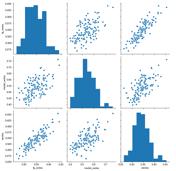
I evaluated model-based wOBA using 2019 data¹ on all qualified hitters. First, I made the pair plot of true wOBA (scraped from FanGraphs, denoted fg_woba), wOBA calculated by my model (model_woba), and xwOBA (scraped from Baseball Savant). Since we’re capturing similar information with these statistics, they ought to be correlated.

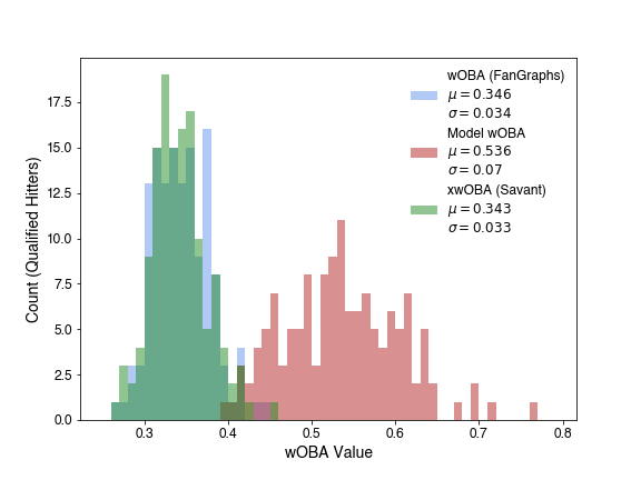
The Pearson Correlation between my model and true wOBA is 60%, while the correlation between xwOBA and true wOBA is 86%. Looking at the pair plot, there does seem to be a difference of scale - overlaying the histograms shows this more explicitly.

This plot accentuates the differences in both mean and deviation for these distributions. This isn’t unexpected however - wOBA is scaled to league average OBP, so that it’s easily parsable. This is a common approach for stat construction in baseball, so for interpretability, we’ll apply this transform to the model evaluations too. For observation \(x_0\), we transform by subtracting the mean of it’s distribution, then scale by the ratio of the standard deviations to set the distribution deviation, then finally add the mean about which we wish to center the distribution.

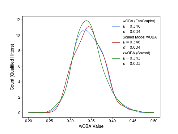
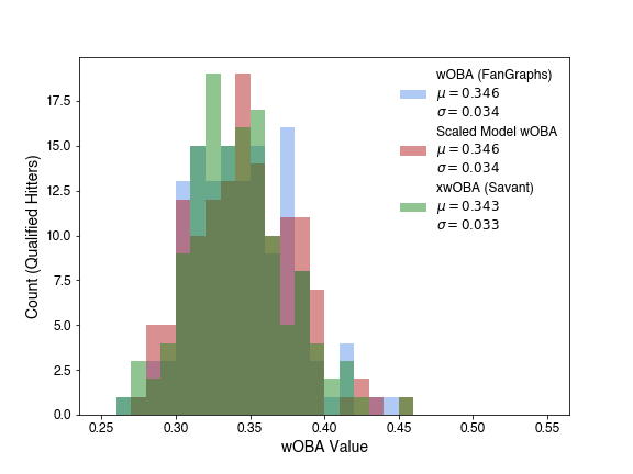
This makes the full distribution of the model-based wOBA now look much more like the other distributions (now shown with kernel density estimate, since 3 overlaying histograms are hard to distinguish²), with no loss of information.

Now that the stats are comparable, we can look at how players are affected by evaluating wOBA using the model, rather than the outcome based wOBA. This plot shows model-based wOBA vs true wOBA. You can scroll over each data point to see which player it represents, along with their xwOBA.

The grey line shown represents where wOBA predicted by the model matches true wOBA (y=x). Players above that line have a better model-based wOBA, players under that line have a better true wOBA.

For those players above the line, the model believes that they have been unlucky in their outcomes, and have disproportionally worse true outcomes with respect to wOBA, based on the hit kinematics, player speed, and park factors. The 5 players with the biggest difference between model based and true wOBA are shown in green: Dansby Swanson, Mallex Smith, Willy Adames, Rougned Odor, and Dexter Fowler. By contrast, the players the model think have gotten the most lucky in their outcomes are shown in red: Jeff McNeil, Anthony Rendon, Ketel Marte, Yuli Gurriel, and Rafael Devers.

Reflection

In Scott Page’s The Model Thinker, he outlines 7 different possible uses for models under the acronym REDCAPE: Reason, Explain, Design, Communicate, Act, Predict, Explore. Not all models are built to meet every component of this acronym - this being a machine learning model, they’re notoriously good at prediction at the cost of interpretability. Through these predictions, it can suggest acting. While the opacity of machine learning hurts interpretability, the development of has served to help explain as well. In the remainder of the post, I’ll go over each of these.

Prediction

This model can be used to predict hit outcomes, using just hit kinematics, player speed, and factors of the park you expect to be playing in. Because of this, it can be used for prediction in several regimes. However, it’s very important to not make out-of-sample predictions, using the model somewhere it isn’t trained to. This model was specifically trained on MLB data, so the domain of applicability is only for MLB-like scenarios. Due to differences in pitching skill, it won’t translate one-to-one to minor league (MILB) data.

Where there is a clear value to prediction from this model would be situations where MLB starters practice against batters. In that case, it doesn’t matter the level of the batters, they could be MLB, MILB, college, whatever, so long as the pitches they’re seeing are MLB-like. If there’s no defense on the field, it might not be clear how these practice hits would translate to real-world scenarios, but this model allows you to predict how the practice would translate to a real game. The scenario I can immediately think of is spring training, where minor leaguers are playing against MLB caliber pitchers - this model would give you a more clear insight about what to expect from the minor leaguers in real game situations.

Acting

The majority of the “acting” available from this model arises in player evaluation. Elaborating from the previous prediction section, being able to understand hit outcomes from players who aren’t necessarily playing in MLB games is a powerful tool, it lets you better understand how to evaluate your players and motivate actions such as when to promote a player.

Further, as shown in the model-based wOBA application above, if wOBA is being used as a metric to evaluate player value, this can provide a more granular version of that, one that removes “resulting” from the equation and filters in some alternative outcome possibilities for the same hits. This would be very useful when doing things like evaluating trades, if you know a player has been particularly unlucky recently and that the model predicts a higher wOBA than the true value, it’s possible you might be able to get a cheaper trade.

Explaining

Through the way in developing this model, there have been several interesting insights, I’ll wrap up with a few:

• Triples are tough to predict. Like, really tough. - This is an obvious statement in passing, but it wasn’t until fighting with this model to get any reasonable triple accuracy that I saw just how dire the situation was. They require the perfect coalescing of correct stadium, quick batter, slow fielder, and a solid hit, which make them incredibly unpredictable. The one case where a model had some accuracy at triples was employing NearMiss re-sampling in post 3, however, to achieve that, overall model accuracy plummetted.

• Hit kinematics get you most of the way there in predicting the outcome of a hit - Beyond exit velocity, launch angle, and spray angle, further variables provided some improvements in accuracy, but not near the gain achieved by the initial three. The feature importance plots in post 2, accented this insight. This is important when considering things like the value of sprint speed - from an offensive perspective, it’s far secondary to a quality hit.

• Focusing on true outcomes loses understanding of underlying skill by neglecting the quality of inputs - In a high statistics regime, such as looking at all hits, there’s going to be many cases where less likely outcomes ended up being the true result; even a 5% probable event sounds low, but still has a 1/20 opportunity of happening, which would occur a couple times every game. Looking at possible outcomes rather than realized outcomes provides a better understanding of underlying talent.

I also encountered some model building insights, that aren’t necessarily insights into the game itself, but still useful to keep in mind, especially for those building models:

• Smart features are just as useful as smart models - I prefer this framing to the often repeated “garbage in, garbage out” mantra. Taking a step back and using informative features is a great way to make sure your model is doing the best it can - take, for example, the favoring of adjusted spray angle over absolute spray angle in post 3.

• Simple questions can lead to useful projects - The launch angle vs launch speed plot color coded by hit outcome was a plot I made quite some time ago, late 2018, because I was curious how to interpret those parameters. That plot sat for about a year, until I was thinking about projects I could use clustering on, and remembered what that distribution looked like, which inspired this project.

• Sometimes your gut model isn’t the right one - I approached this problem thinking it’d be a neat way to employ k-Nearest Neighbors clustering. However, one of the first things I discovered in post 1 is that tree based methods do better than k-NN - keeping an open mind to alternative models is good, test as much as you can. This calls back to the “fox vs hedgehog” metaphor to approaching forecasting, popularized by Tetlock - hedgehogs develop fixated on one model, where foxes consider different angles, which usually leads to more accurate predictions.

I’ve spent quite some time fleshing out this model, and I think I’m putting it to rest (at least for now) to work on other projects, I hope that these posts have been useful, interesting, or informative! Thanks for reading.

The code for this post can be found in this Jupyter Notebook.

Footnotes

[1] The model was trained and tested on 2018 data, so for a “foreward prediction,” I elected to evaluate on 2019 data.

[2] Proof:

• 2023 1
• 2022 2
• 2021 1
• 2020 10
• 2019 8
• 2018 3
• 2017 1