Box Score Thoughts: Tempering Run Expectations from Hits

Background

About a year and a half ago, I was reading box scores one day and saw a game with a ton of hits, but very few runs and was surprised at this. Then I paused to wonder - should I be surprised? How should I expect these to scale? I’ve been watching baseball for a long time, but I wondered if my a priori expectations here were miscalibrated.

That night I quickly put together an ad hoc analysis which I posted here, but never quite felt proud about; the methodology wasn’t great. Rather than take it down, I’ve worked to improve it (the original post appears in it’s entirety at the bottom of the page). The ultimate question I wanted to answer is “conditional on the number of hits, what should I expect for number of runs?” To do so, I’ve developed a model with the primary goal of creating a better baseline for my personal expectations.

Data

Just looking at the raw distribution of this parameter space for 2018 data:

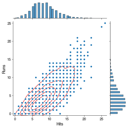
There’s a lot to note here. First, most of these points represent many, many games, and this distribution is overwhelmed by the data in the lower corner of the distribution. This is emphasized both by the density contours shown in red and the histograms on each axis. However another key feature here is that width of distribution spreads out as the number of hits increases. This is a quality known as heteroscedasticity, a word which I will never be able to spell right on the first try. It’s important to note that one of the assumptions for traditional linear regression is that it’s homoscedastic, so this assumption is violated in this case.

Model

After considering several different ways to model this, I ultimately used a Bayesian linear regression model (using PyMC3), with an extra trick to manage the heteroscedasticity. While standard linear regression assumes constant variance, instead I used a linear model for both the mean and variance of the outcome variable. That is to say, we assume that the number of runs is normally distributed, in which both the mean and variance of that normal distribution scale linearly with respect to the number of hits. Expressly, the model is:

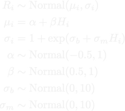
Here you can see two linear models for each of the parameters of the normal distribution. I’ve applied a trick to \(\sigma_i\), the standard deviation, transforming the linear model with an exponential function in order to ensure that the value is positive. In terms of a directed acyclic graph, this looks like:

This model is then conditioned on the data from 2018, and yields the following distribution, with the 1 and 2 standard deviation bands shown.

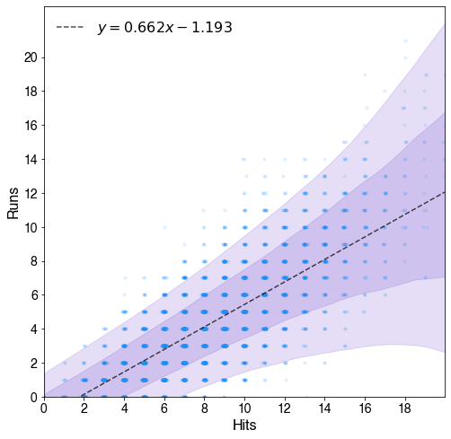
This model has good coverage of the data, and takes into account heteroscedasticity pretty well. Several other models were considered - a standard normally distributed linear regression, a more robust regression using a Student’s T-distribution, and this one proved to be the best (in terms of information criteria metrics).

Takeaways

The takeaway here is that while we expect the number of runs to scale with the number of hits, the range we expect should be very broad, even broader than my default expectations. With 5 hits, for example, we can be 68% confident that there will be between 1 and 3 runs, but our 95% credible interval is anywhere from 0 to 5 runs, so neither of these outcomes should surprise us. It’s not until 8 hits that 0 runs falls out of the 95% credible interval - considering more than 1/8 hits in 2018 were home runs (13.6%), one of those probably automatically converts to a run, so this isn’t entirely surprising.

I think the points of reference I will keep in mind from this in future baseball watching is that at 5 hits, 0 runs falls out of the 68% credible interval, and at 6 hits 1 run falls out. Teams that don’t meet those benchmarks are in the lower 34% of run conversion with respect to hits. On the flip side, teams producing more runs than hits are all outside the 1 sigma band. Again I can use 5 hits as a reference here - at 5 hits, 4 runs puts a team in the upper 34%, so I can keep in mind \((N-1)\) runs for \(N\) hits as a well-above average result. At 9 hits, this becomes \((N-2)\).

The code, along with additional plots, model comparisons, and more is available on my GitHub in this Jupyter notebook.

Original Post - June 23, 2019

Recently after seeing a box score with many hits but no runs, I’ve been thinking a bit about run expectancy based on the number of hits in a game. Obviously these are going to be correlated, but I was curious, how strongly, and how well you could predict runs given number of hits.

I went and looked at 2018 data for runs scored based on number of hits and did a linear regression:

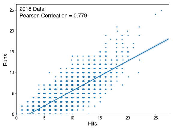
As expected, the Pearson Correlation is 0.779, which falls under “strongly correlated.” In an attempt to try to get to some prediction method, I calculated the mean at every hit value, and plotted those values, then tried to fit that data.

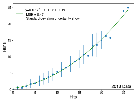
Looking at just the means, a linear fit does not match the data well, so a polynomial fit of order 2 was used, which does. The coefficient on the x² term appears small, but once you get to 6 hits, it raises the expectation by an additional run. Once you add standard deviation uncertainty lines to this plot though, you could see that within the 68% confidence interval of 1 sigma, a linear fit could probably work just as well to this data.

• 2023 1
• 2022 2
• 2021 1
• 2020 10
• 2019 8
• 2018 3
• 2017 1