Classifying MLB Hit Outcomes - Part 2: Optimization

Optimizing a model to predict hit outcomes

In the first part of this series, I looked at how launch angle and exit velocity translate to MLB hit outcomes using data from 2018. To predict the outcome of future hits, several models were investigated including k-Nearest Neighbors, a gradient Boosted Decision Tree, and a Support Vector Classifier. Of these three, the tree-based method was the most accurate, correctly classifying 77.7% of hits.

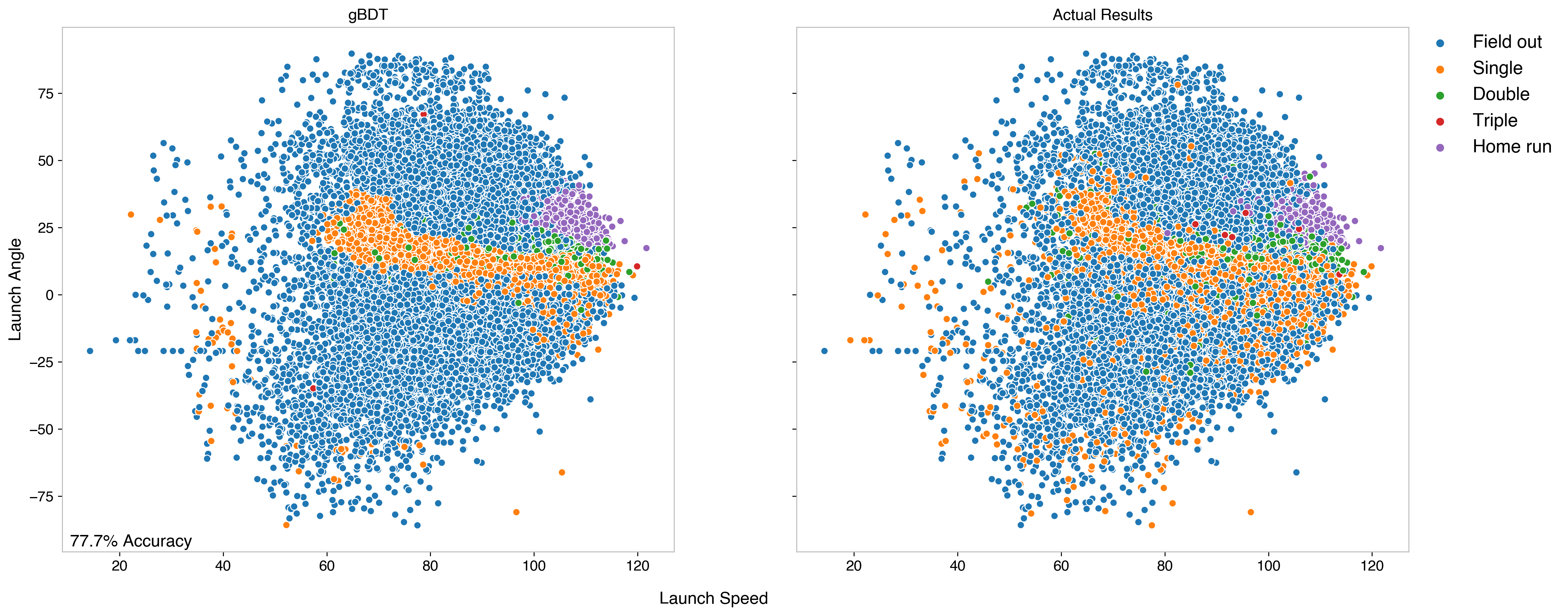
That was an out-of-the-box model from Scikit-learn, with just 3 inputs describing the kinematics of the ball, namely the launch angle, spray angle, and exit velocity. In this post, I’ll extend that work by looking at a couple of ways to improve on the model, through incorporating new inputs and optimizing the model parameters.

Studying Additional Inputs

Looking at previous confusion matrices, the largest immediate flaw in the model is that it cannot classify triples. This is understandable, since triples are a tough to predict: they need some combination of the right hit, the right park, a fast enough player, or a slow fielding attempt. When considering new inputs, this was at the forefront of my mind. The two major factors I’ve tried to incorporate into this model are park effects and player speed, which I’ve tried to encapsulate through adding park factors and sprint speed as inputs.

Park Effects

Hit outcomes are dependent on the park, particularly when it comes to home runs and triples. This can vary for several reasons, such as park dimensions (e.g. the infamous 421’ Triples Alley in San Francisco), weather/location (e.g. the elevation of Coors in Denver or heat in Arizona), and features in the park (e.g. the Green Monster in Fenway).

This has been studied and captured into what’s known as Park Factors. These are derived to standardize stats for batter-friendly vs pitcher-friendly parks, since in general player evaluation we want to understand how good a player is independent of stadium. Several levels of granularity for park factors are available, varying from a general “is this park batter or pitcher friendly” factor to a more specific “how much more likely is it for a left-handed batter to get a double in this park” factor.

When considering as an input, I selected to use more granular park factors: the propensity of singles, doubles, triples, and home runs for a batter with given handedness in the ballpark the game was played in. Selecting to add park factor by hit-type is important to segment out HRs from triples, rather than just offensive from defensive. Adding by handedness is important to account for the asymmetry of several fields.

In terms of the model, this added 4 new features, 1B park factor, 2B park factor, and so on corresponding to the batter’s handedness. Since this is evaluated on 2018 data, I assumed park factors from 2017 were known and used values from Fangraphs. I retrained the BDT using the park factors and original hit parameter inputs, now using the XGBoost framework (a better and more flexible framework for gBDTs). I’ve also increased the maximum depth to 12 to allow the model to take advantage of new features.

By increasing depth, the accuracy improves marginally from the previous 77.7% to 77.8%. Then, by adding the park factors, this increases up to 78.2%. Also notably, it now is predicting a handful of triples accurately - 6 correct of the 432 in the dataset.

Player Speed

Another factor in hits is how fast the player can run. With respect to extra-base hits, slow players generally get far fewer doubles and rarely ever get triples. Fast players also have the opportunity to beat out close plays at first more often than slow ones, which also makes a difference between singles and outs.

To add this information into the model, I included player sprint speed from the 2017 season¹, which is available at Baseball Savant. I made a small quality cut, requiring at least 10 attempts. Players that either did not play in the 2017 season or who failed that cut were assigned the mean sprint speed value.

Adding this information only marginally improves the model, improving accuracy by just 0.02%. Most of that improved accuracy comes from better predicting doubles, however this model also predicts 5 triples correctly (and only one of those triples was the same as the correctly predicted one from the park factor model).

Combining all new features

So far, we’ve looked at improving the BDT through adding park effect information and sprint speed to the original hit kinematic variables independently. Now, we can put those together and see how this model performs. For those of you counting along, this model has 8 inputs: 3 hit parameters, 4 park effect variables, and sprint speed.

Putting all this information together gives a slightly better model than any prior ones, at 78.24% accuracy. Ultimately this gain is still small, but still of interest: this model now correctly predicts 10 triples. Obviously, while better than before, this isn’t an overwhelming success, but it highlights how difficult triples are to predict. The model also is better at predicting doubles (from 46% to 50%) and home runs (from 73% to 76%).

Model Optimization

Now that the inputs have been defined, the model itself can be optimized. In this post, I’ll do so via optimizing the hyperparameters, variables which are not a part of the data, but of the model and training process itself. These are fixed before training, and involve things like depth of trees, number of trees, learning rate, and so on.

Since we’re already working within the margins, an exhaustive grid search of many hyperparameters is overkill; it’s a bit meaningless to squeak out that last 0.001% accuracy when we want a generalizable model. Rather, I’ve done a search over a few key hyperparameters², with plots for transparency and interpretability.

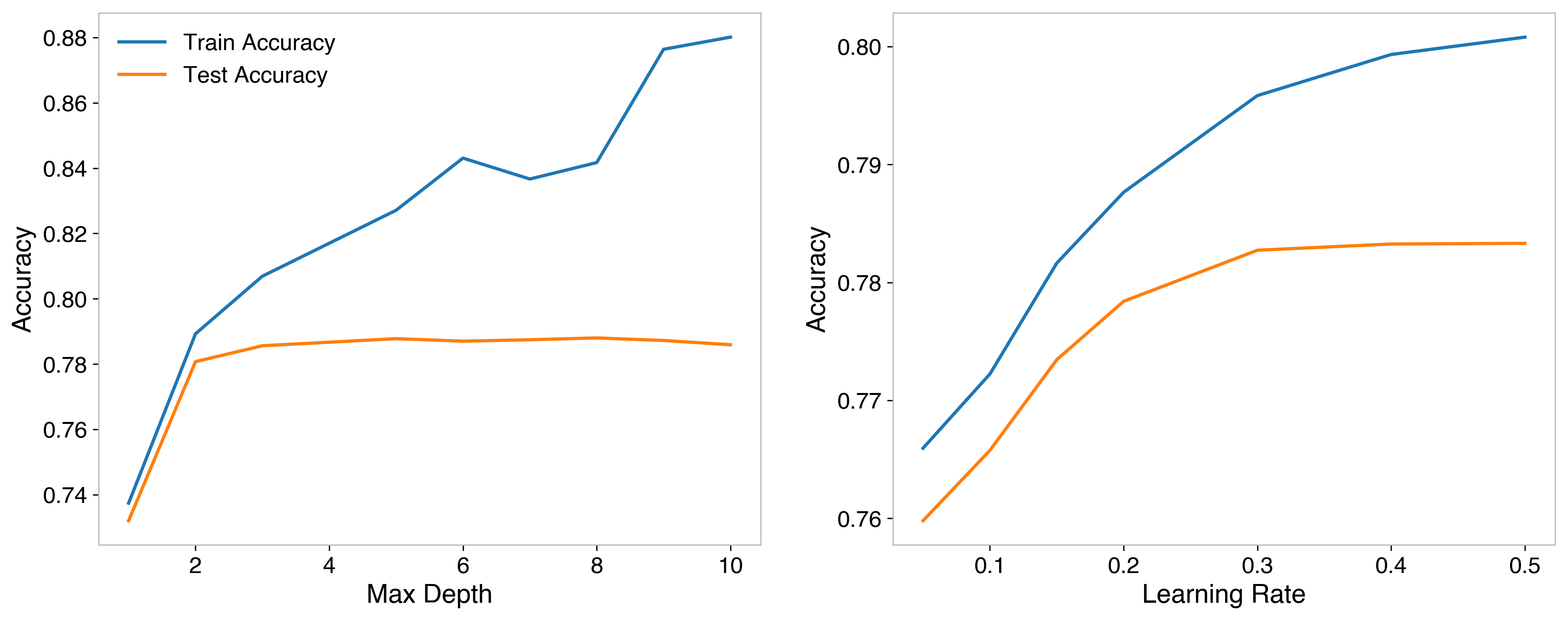
The two hyperparameters we’ll look at are max_depth and learning_rate. The max_depth parameter is pretty easy to envision: BDTs are composed of trees (think a flowchart) which segment the data based on input features, and the depth is the how many successive cuts can be made for any of the trees. This makes it one of a handful of “stopping conditions.” Too shallow of trees will not take full advantage of the input features, too deep will cause overfitting and not allow the model to generalize to new data.

The learning_rate is a bit more abstract³. After building an initial tree, the model identifies misclassifications, and upweights them in the following tree, and performing this over and over is known as boosting. The learning rate is a regularization technique, that shrinks the weights in successive trees by a factor in order to make the process more conservative. This effectively “dampens” the effect of additional trees and makes the model less prone to overfitting.

I trained models first finding the best possible depth, all other hyperparameters kept the same, then the best learning rate (using the best depth found before). The best value for maximum depth was 5, beyond that the accuracy on testing data doesn’t improve, and it just becomes more overfit on the training data. For learning rate, accuracy leveled out on training data at 0.3.

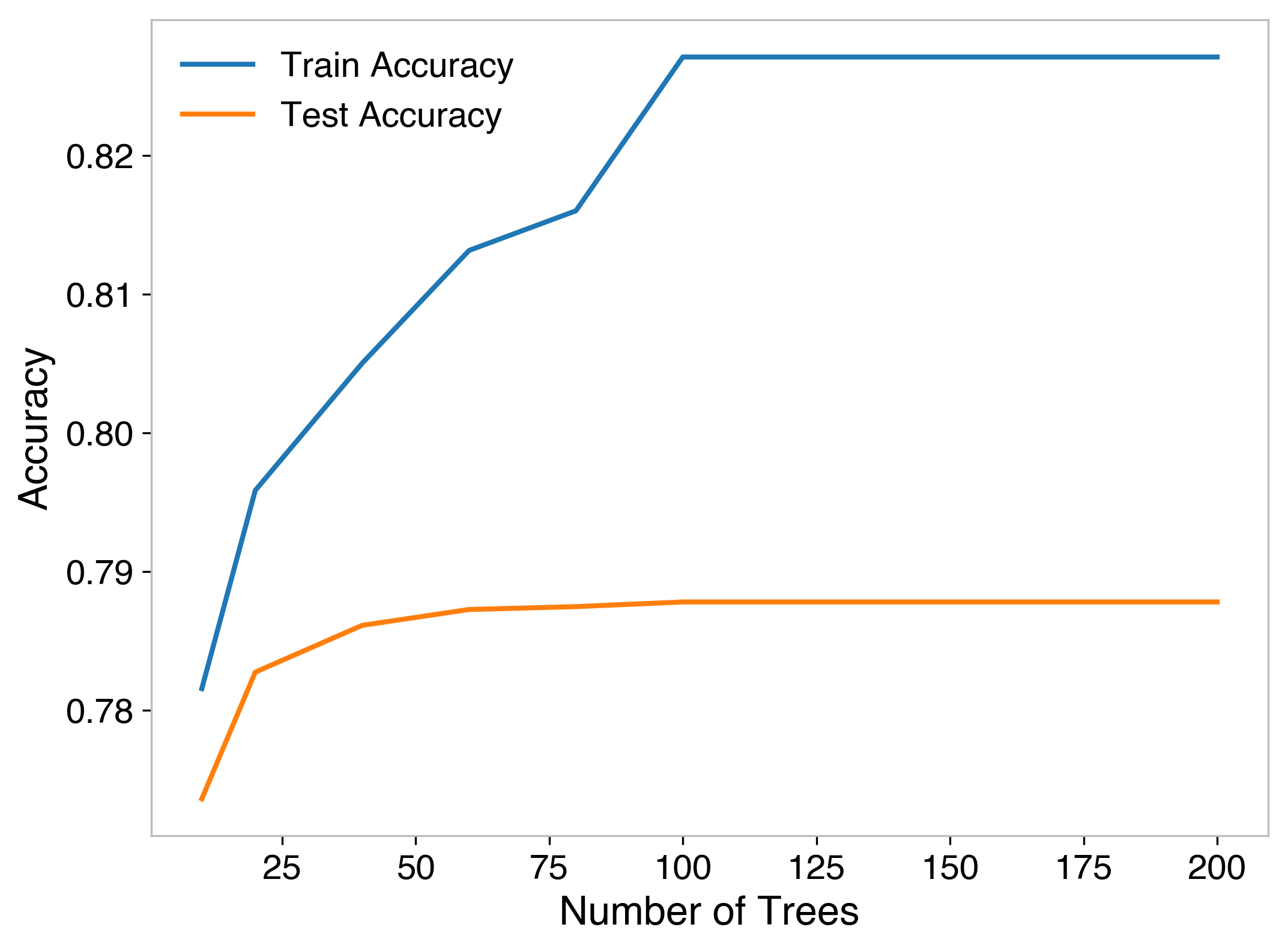
As far as number of trees used, another important hyperparameter, I employ “early stopping.” If the model hasn’t improved for 30 trees, then it will stop producing additional trees. The number of trees is then set to a large value, I chose 200, intending to stop before this number. To verify this, I trained models at various values for maximum number of trees and find that it hits this wall by about 100, so this configuration is fine for that hyperparameter. The final model looked at 121 trees in training, meaning there were not additional improvements beyond the 91st tree.

Finally, I built a model using these optimized hyperparameters, and generated the confusion matrix again.

The model has improved to 78.78% accurate, which is a nice improvement over the prior models. Most of that improvement comes from better predicting singles and home runs. It does make sense that the optimization prioritized these, since singles are the most dominant non-out hit type - in the testing data, there’s 12,762 singles compared to 7,439 other hits (4,184 doubles, 432 triples, and 2,823 home runs). Unfortunately, this comes at the sacrifice of triples - the new model moves down to just 3 predicted accurately.

Summary and Future Work

Ultimately, this is a whole lot of work for a very small gain, which raises the question if this work was actually worth the effort, or if this was just a way to burn quarantine hours that I could have spent playing Animal Crossing. From a model building perspective, I think it’s fair to see this as not-so-useful, but from an insight and understanding perspective, there’s some interesting things to learn from this study.

In adding new variables that I assumed would be useful in helping predict outcomes, I found less improvement than expected. From this, we can learn that the most useful predictors of hit type are the kinematics of the hit itself. Player speed, park effects are subdominant effects compared to how the ball was actually hit. In experience, this does make sense - slow players still have jobs and can be very productive batters, after all.

Looking at the feature importance of the final model can confirm this; all of these features are far less useful than the original 3 we started from. The feature importance shows either the improvement in accuracy by cutting on a feature (gain), or a count of how many times a feature is cut on (weight). By both metrics, the hit kinematics are far more important in the prediction than any of the other features.

An additional upshot of doing this work is that the model does predict a handful of triples correctly, and sees an improvement in home runs and singles as well. Future posts will start looking at ways to improve further, investigating methods of balancing out the dataset, so knowing that these additional features help in that prediction gives a better starting point in approaching that problem.

The code for this post can be found in this Jupyter Notebook.

Appendix - A Multi-Level Model Approach

In the development of this, I considered developing a multi-level model to improve the performance. The basic idea was to have one binary classifier to identify “is this a hit or not?” and one multiclassifier to identify “what type of hit is this?” I liked this idea, since it takes the single very imbalanced classification problem and converts it to a balanced binary classification and a somewhat less imbalanced multiclassfication. Additionally, I thought different models might perform better at one task over the other, and this gives that flexibility.

I found that in both cases the BDT still performs the best, the left showing for the binary classifier (hit or not), the right for the multiclassifier (what type of hit). There’s not really a strong motivation to change the features in one over the other: the hit kinematics, park factors, and player speed are all relevant to both questions, so the same features are used in each.

If both models are BDTs, and both have the same input features, there shouldn’t be an advantage in splitting the model in two stages in this manner (provided there are sufficient trees, verified above). Nonetheless, I went ahead and tried it, first optimizing the hyperparameters for each classifier.

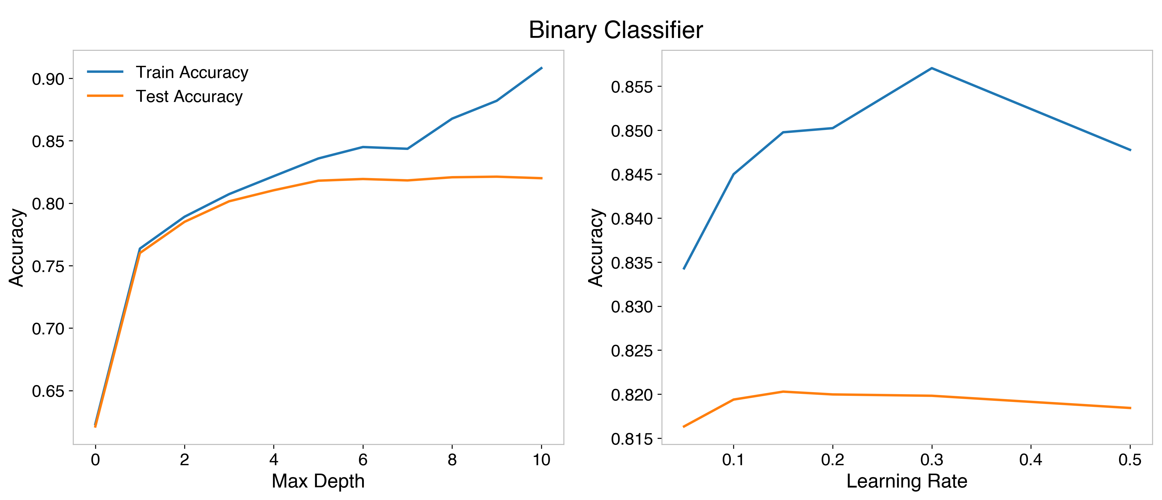
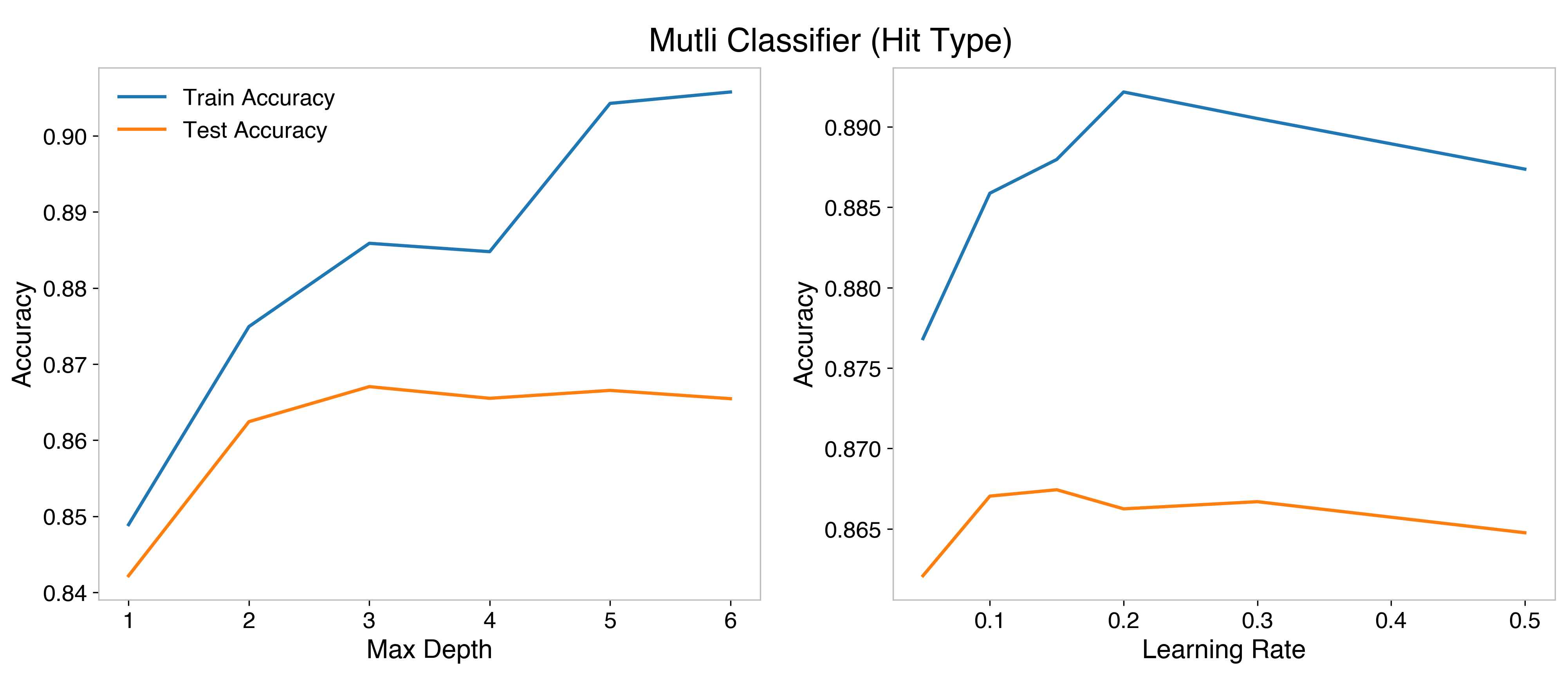
The binary classifier is optimized at depth 6, and learning rate 0.15. The multiclassifier is optimized at more shallow trees, just depth 3. A learning rate of 0.15 is optimum for it as well.

Additionally, I scanned over the probability distribution output by the binary classifier, to find the most accurate point to draw the distinction of what I consider a hit. The left plot shows the probability score the BDT assigns on the whole testing set, the right shows the overall accuracy if the cut to distinguish “hit” is made at that point.

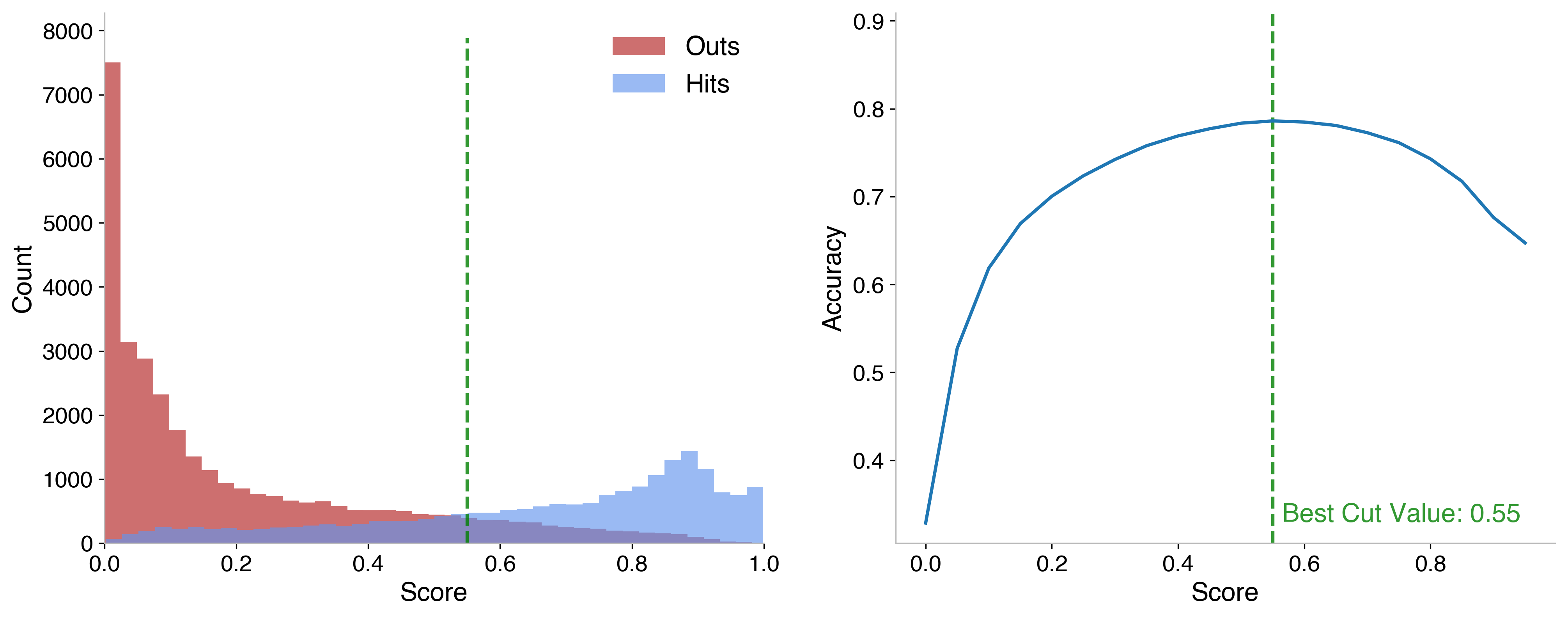
It was found to be optimum at 0.55 (expected to be around 0.5, so this is good). Instances higher than that are considered hits and evaluated by the multiclassifier, lower than that are classified as field outs. Then, drawing the confusion matrix, I find that, in fact, this model does marginally worse.

Granted, we’re still looking at differences of tenths of a percent, so this loss isn’t incredibly meaningful. When I consider resampling approaches in the upcoming posts, though, I’ll keep this model in mind since it will reduce the number of instances that fall into the imbalanced dataset.

Footnotes

[1] An earlier iteration used stolen base metrics, rather than sprint speed. I investigated using attempted steals, successful steals, number of times caught stealing, and SB rate. The two that gave the best performance increase were attempted steals and number of times caught stealing. At the end, adding sprint speed explicitly performed better than including these, so the final model used sprint speed.

[2] Hyperparameters are somewhat correlated, so optimizing sequentially is not ideal, and this is why a grid or randomized search would be better for overall performance. However, this leans toward less transparency - I’d like this to be digestible to the reader (and myself!). Also, since we’re seeing improvements of hundredths of a percent, a grid search won’t add much on top of just tuning the key parameters, a quick study showed improvement was at the order of hundredths of a percent.

[3] For those of you with deep learning experience - this differs from the learning rate typically in gradient descent, in which it is the step size of the gradient descent algorithm.

• 2023 1
• 2022 2
• 2021 1
• 2020 10
• 2019 8
• 2018 3
• 2017 1