Gauging Home-field Advantage in 2020

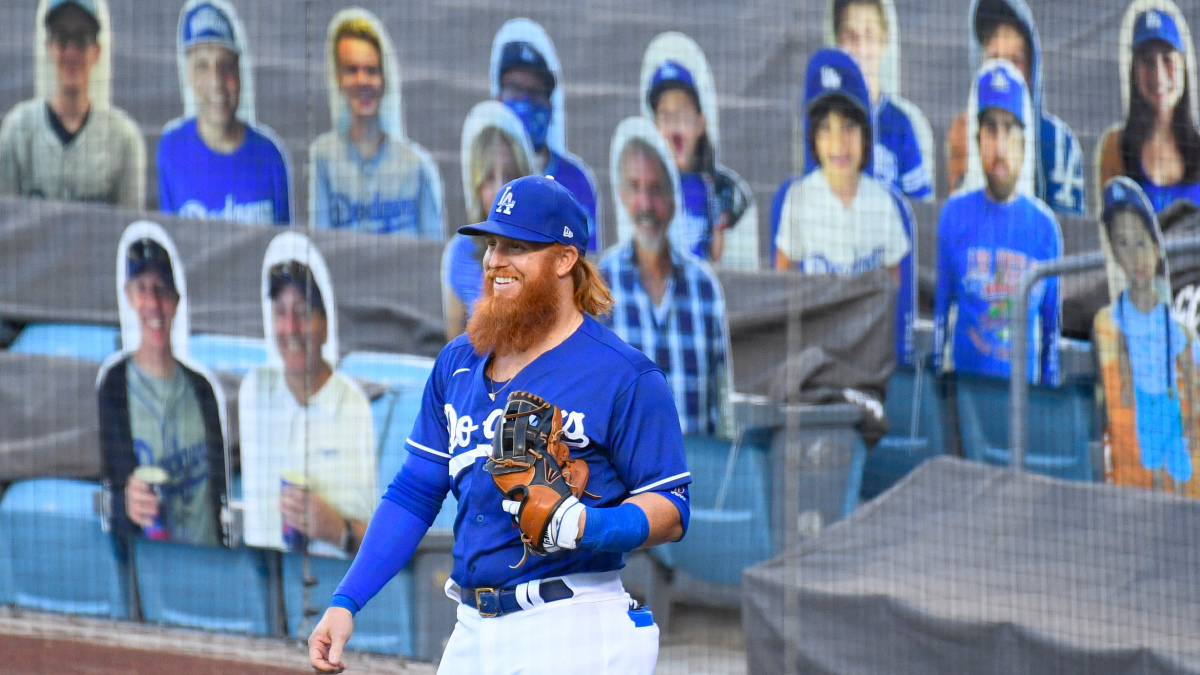
As a result of the COVID pandemic, baseball in 2020 looked very different. Several new rules have changed the appearance of the on-field game, however I’ve been interested in a change off the field: the impact of fans on home-field advantage. As a result of the pandemic, cardboard cutouts and simulated stadium sounds have replaced human fans, which begs the question - with no fans, does home-field advantage still exist? If so, to what degree?

There’s been quite a bit of writing about this, with mixed results. Ben Lindbergh at The Ringer argued that home-field advantage did persist in 2020, while Mike Petriello at MLB said the opposite in August, citing the 50.5% home winning percentage. Tyler Kepner at the New York Times goes as far as to argue that home-field advantage never existed. I sought to understand what we can truly say about home-field advantage given the abbreviated 60-game season.

Methodology

The goal in this study is to estimate the degree to which home-field advantage exists, which will be estimated by a run advantage, or “how many more runs we can expect from a home team compared to an away team.” In order to estimate this, I’ll be doing parameter estimation via Bayesian inference. This means that we assume there is some underlying “true home-field advantage,” and the run advantage in each game is a realization of a random sample of this parameter.

To do this estimation, I developed a generalized linear model to predict the number of runs a team will produce in a game. The outcome variable of “runs” is a count value, which must be modeled with a discrete distribution, since it only takes on integer values. I’ve used a negative binomial (or gamma-Poisson) distribution to model this variable. The negative binomial distribution is a Poisson distribution that assumes each count observation has its own rate, resulting in 2 free parameters, which allows for more flexibility than the traditional Poisson distribution.

Next, I assume the mean of the negative binomial comes from the log of a linear function with 4 predictors. I assume the scoring in a game is impacted by 4 sources:

• \(S_i\) - The team’s strength
• \(P_i\) - The opposing pitcher’s strength
• \(H_i\) - The league-wide home-field advantage
• \(\tau_{\text{STADIUM}[i]}\) - Park effects for each individual stadium

In order to model team and pitcher strength, I’ve used values from an ELO rating system, which calculates relative skill levels in zero-sum games, under the assumption that performance is normally distributed. Luckily, FiveThirtyEight maintains game-wise ELO values for each team and adjustments for opposing pitcher strength, so these were used as predictors. Additionally, there’s different run-scoring environments in various stadiums, so the model controls for that by adding a categorical intercept for each individual stadium. Last being a linear model, I also have an intercept \(\alpha_i\).

Using Bayesian inference means prior expectations must be assigned to each parameter. I’ve tried to do this fairly conservatively by giving wide priors (remember, since the logarithm of the linear function is in the model, so these terms are exponentialed). I assume team strength and pitching will be the two dominant factors, so I’ve given them normal distributions with a standard deviation of 1. Next, the home-field advantage and park-effects are far less dominant than the team strength, so these predictors are given smaller normal distributions, a standard deviation of 0.1. Last, the second parameter of the negative biomial distribution, \(\alpha_i\), is the gamma distribution parameter. This value controls the spread of the distribution - it must be positive, so I gave it a flat prior over a very wide range of 0 to 10.

In it’s completeness:

Data

As mentioned before, I’ve used the ELO CSV from FiveThirtyEight. For the first part of this analysis I’ve selected just data from the 2020 regular season, which occurred at non-neutral sites. The team ELO and pitcher adjustment values were standardized (mean moved to 0, standard deviation to 1). Home team is saved as a boolean value, 1 for home and 0 for away, and stadium is saved as the home team in any given matchup, which is encoded into an index ranging from 0 to 29.

Model Sampling

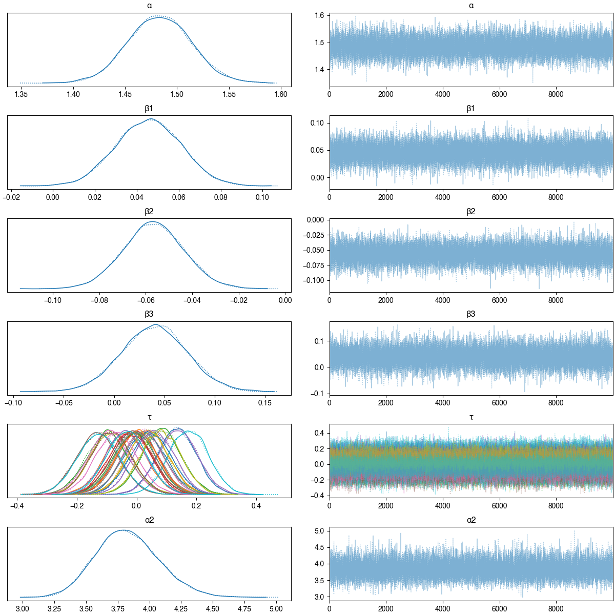
The model was constructed using pyMC3, and I’ve drawn 20,000 sample parameter sets from the posterior distribution¹ - possible parameters which may have generated our data given the priors and conditional on the runs scored in 2020. Using this, we can draw predictions from our model:

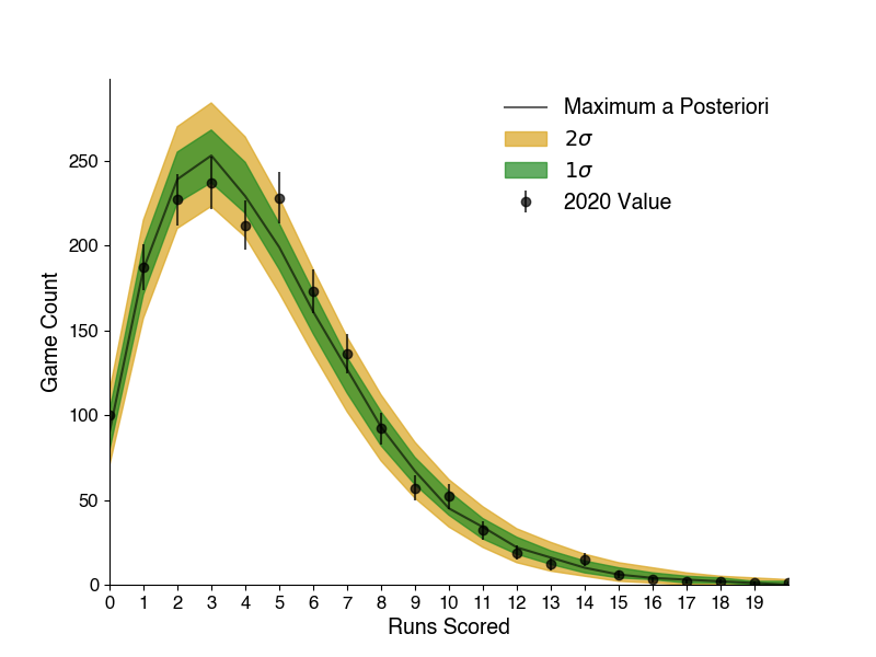
The inner green band on this plot covers the 68% (1 standard deviation) most common outcomes, the outer yellow band encompasses the 95% (2 standard deviations) most common. The most-likely value is shown with the solid black line, and the 2020 actual result is shown with the markers (Poisson errors are shown). Here we can see this model covers our data quite well, all of the true values lie within the \(2\sigma\) band, with just a couple of error bars slightly falling out. Two other useful sanity checks to make sure the model works as intended: the most likely value for the impact of team strength on runs is positive (0.05) and the opposing pitching is negative (-0.06), meaning the model confirms stronger teams produce more runs, and good opposing pitchers suppress runs - which is what we would expect.

Evaluating Home-Field Advantage

Now that we have a model that can predict the runs a team will score, we can use this model to generate new predictions. For each of the 20,000 parameter sets, a new season is simulated - 30 home games and 30 away games for each of the 30 teams. Then we can compare the mean score of the home games to the away games for all teams in the league for each simulation to understand the home-field advantage.

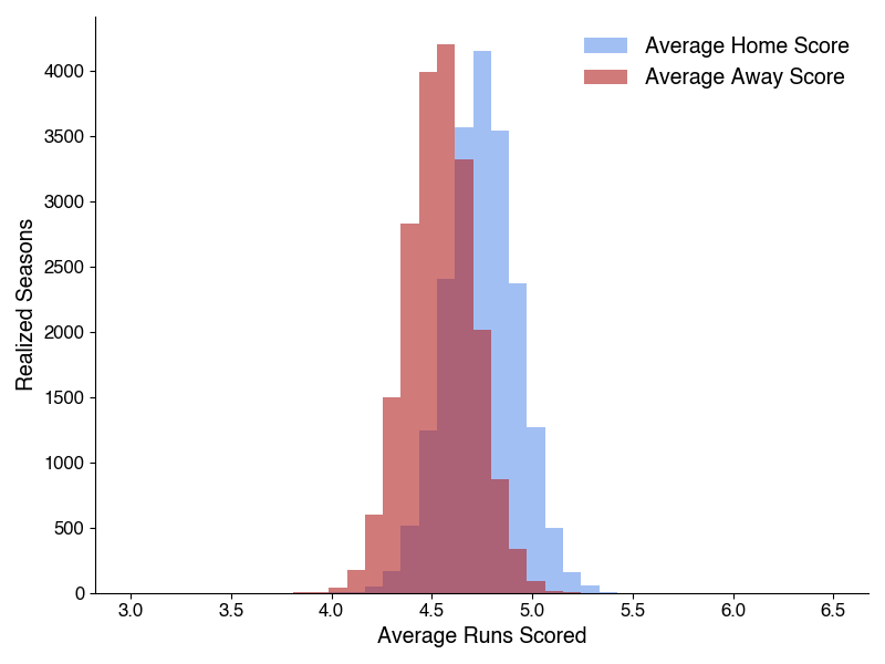
These histograms show each simulated season’s mean home and away scores, and the peak of the home scores lies above that of the away scores - the model shows home-field advantage does seem to exist, to some degree. We can then take the difference of these two distributions to quantify how much.

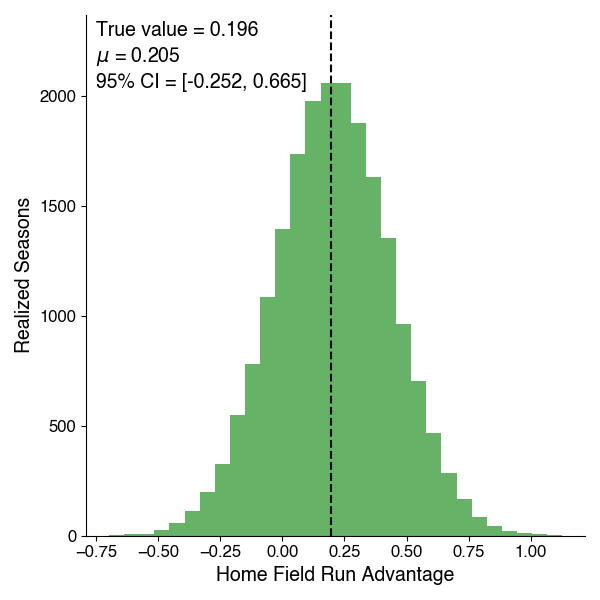
The mean of this distribution lies at 0.205, indicating that given this model, the home team most likely gets an advantage of about 1/5th of a run when playing at home (this could be interpreted as “one extra run every 5 games” for those uncomfortable with fractional runs). The true value in 2020 is also shown, at 0.196. The 95% credible interval here spans from -0.252 to 0.665, which means this analysis can’t necessarily rule out the idea that no such effect does exist, nor can the analysis rule out that it was worth half a run in 2020. However, 81% of this distribution lies above 0, so we can say there’s an 81% chance that the home-field run advantage exists and is a positive value.

Comparing to Previous Years

To get an idea of how this benchmarks against previous years, I re-ran this analysis for every year since 2014. The model and approach were held constant, the only difference was conditioning on each year’s respective data set. To see if home-field advantage in 2020 was different, I plotted the predictions for each year, looking at the 95% credible interval:

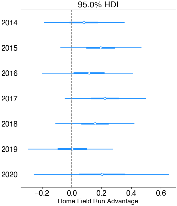
Note that 2020 has a wider prediction interval due to the shortened season: less data makes the model less certain. From this plot, it’s tough to say anything entirely definitive about home-field advantage - just like in 2020, we can’t rule out 0 at the 95% CI for any given year, nor can we rule effects as large as 0.4 runs for most years. 2017 comes the closest, with 94.6% of the posterior lying above 0. However, In all years but 2019, the vast majority of the probability distribution lies above 0, so we can be reasonably confident that there’s a positive home-field advantage effect on run scoring.

Summary

Going back to the claims, it seems that we don’t quite have enough evidence to rule out any claim definitively. I would argue it’s hard to justify that home-field advantage never existed, since each of these years have a large portion of their probability interval being a positive value, but technically all could be consistent with 0. Otherwise, home-field advantage at the run-level in 2020 doesn’t look all that dissimilar to prior years - the way the prediction interval lies, it’s more consistent with other years in which it took a positive value. The most likely value per this analysis is about 1/5th of a run, so I would agree most with Lindbergh’s claim that removing fans did not remove MLB’s home-field advantage.

Code for this analysis is available on my GitHub.

Extending this work

In this analysis, I’ve considered home-field advantage as a league-wide phenomena, implying every team has the same run advantage while playing at home. This assumption worked for the context of the study, since the lack of fans was league wide. However, it might not be entirely true. While at some level stadium effects should cover variation in stadiums themselves, it could be that some teams have a higher home-field advantage. Breaking this data down even further into the team level would cause data sparsity though, only 30 home and 30 away games per team - this is something that could justify a hierarchical modeling approach.

Further, considering home-field advantage as an independent analysis for each year isn’t entirely justified, there ought to be some continuity in value between years. However, it’s dependent on run scoring environment (e.g. the recent home run surge will likely make an impact), so a time-varying model could also be considered in order to take advantage of year-to-year data while accounting for temporal variation.

Last, this analysis looked at the run-level effect of home-field advantage, but a more granular study could be performed. The Lindbergh piece cited above studies at-bat level data, which would provide more statistics to perhaps give stronger claims on how home-field advantage affects at the player level.

Footnotes

1) Model converges nicely, trace plot:

• 2023 1
• 2022 2
• 2021 1
• 2020 10
• 2019 8
• 2018 3
• 2017 1