Classifying MLB Hit Outcomes - Part 1: Model Selection

Understanding Launch Angle and Exit Velocity

In 2015, MLB introduced Statcast to all 30 stadiums. This system monitors player and ball movement through the combination of two tracking systems: a Trackman Doppler radar and HD Chyron Hego cameras. This has provided a wealth of new information to teams, but also has introduced many new terms to broadcasting parlance. Two specific terms, exit velocity and launch angle, have been used quite frequently since, with good reason - they’re very evocative of the action happening on the field.

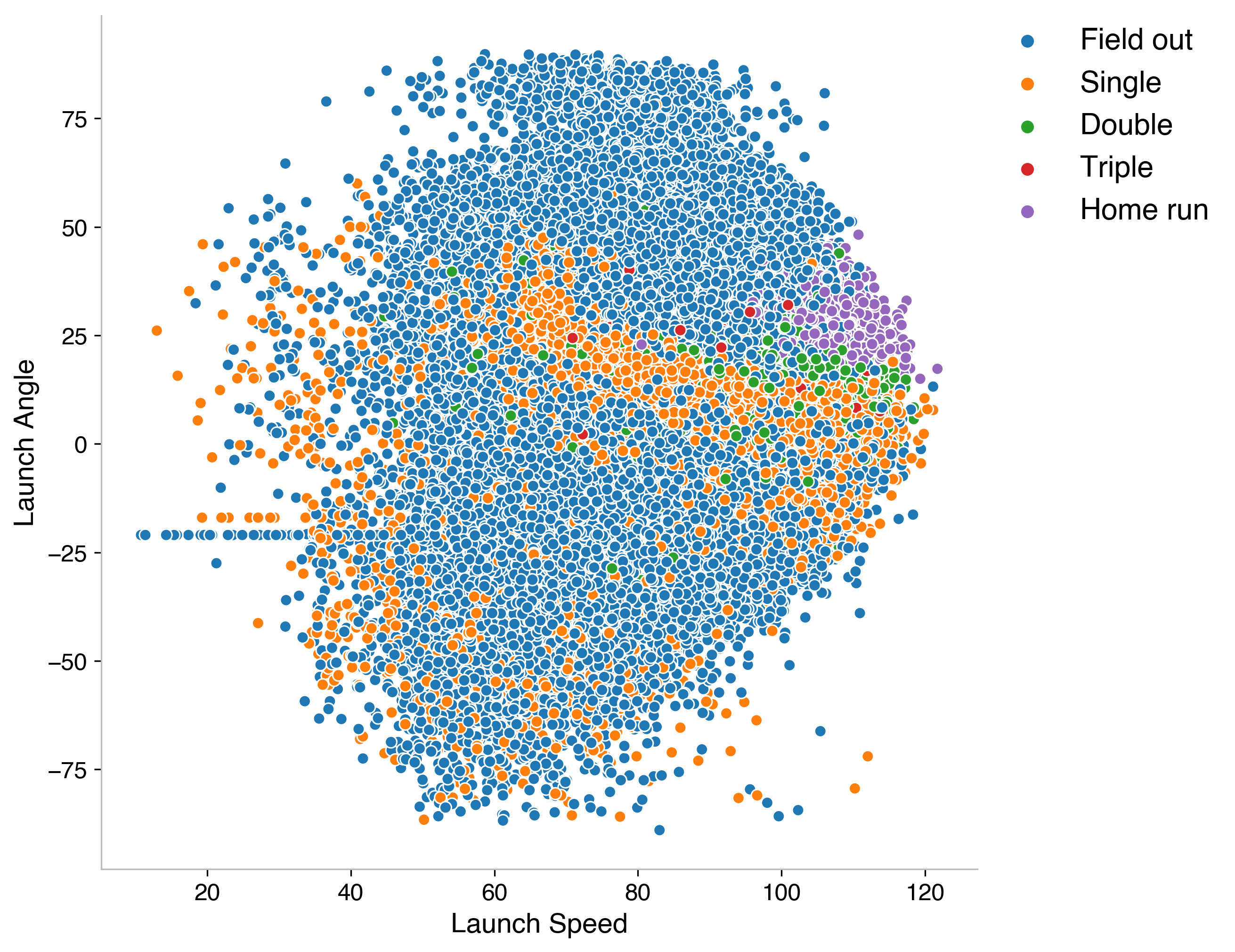
The exit velocity is the speed of the ball off of the bat, the launch angle is the vertical angle off the bat (high values are popups, near zero values are horizontal, negative values are into the ground). When these started becoming more popular, I found myself thinking quite often, “how do I know if this is good or not?” With exit velocity, it’s fairly easy to conceptualize, but less transparent for launch angle. This led me to try plotting these two variables using hit outcome as a figure of merit. The shown chart uses data from the 2018 season.

There are some macro-trends of note here:

• There’s a “singles band,” which stretches from roughly 45 degrees at 65 mph to -10 degrees beyond 100 mph. The former represents a bloop single, the latter is a grounder that shoots past infielders, and this band as a whole encapsulates everything in between.
• There’s a pocket for doubles, which occur primarily for hard-hit balls (over 85 or so mph), generally hit slightly above the horizontal, between about 5-20 degrees. These correspond to hard hit line drives, specifically that make it to the deep parts of the outfield.
• There’s an even more defined pocket for home runs, these have to be above the horizontal, but not too much: between 12 and 50 degrees. They also have to be hit at least 80 mph.
• Triples are too rare to make any meaningful comment on. They’re heavily park and player dependent.
• There’s a considerable amount of stochastic singles at low launch speed. These can correspond to things like bunts against the shifts, infield hits, etc.

Employing in a Prediction Model

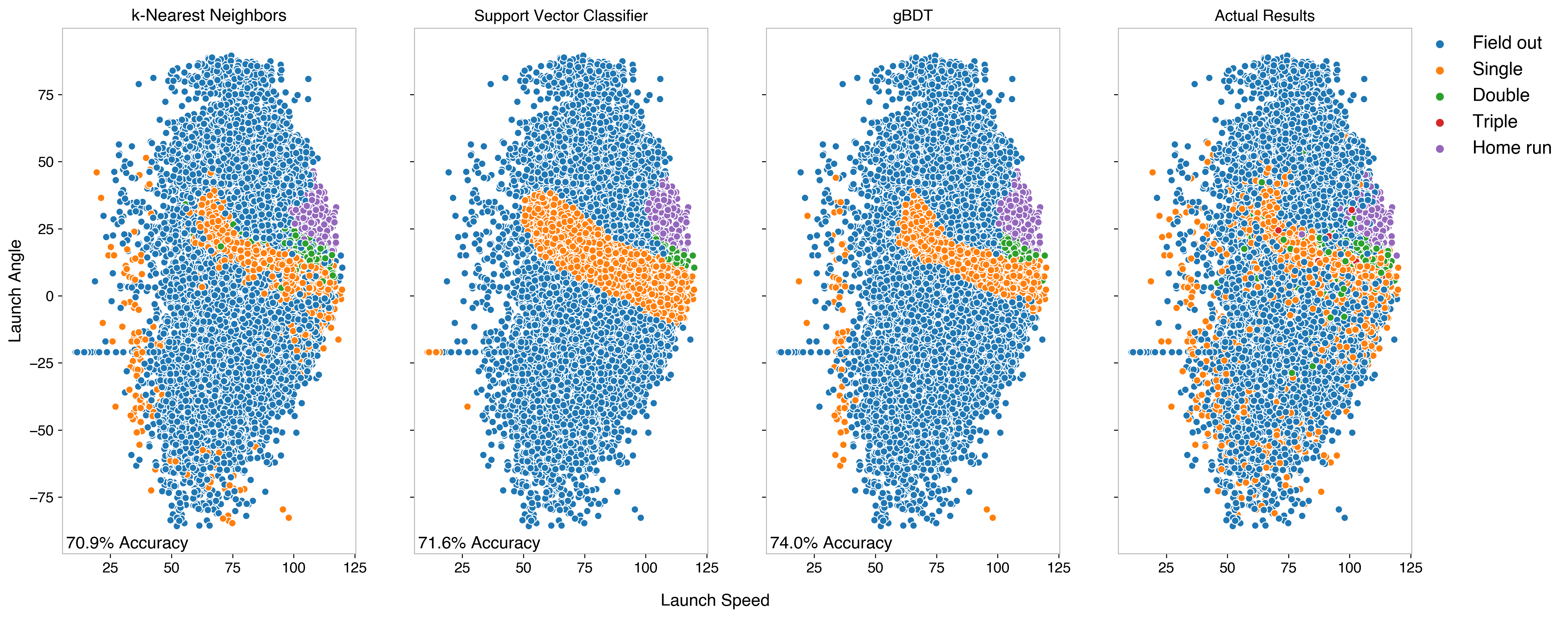
A while later, I came back to this plot and considered how one might model these trends. The pockets immediately made me think about k-Nearest Neighbor clustering, which was my first attempted model. I also took a look at some other classification models. The models I’ve investigated here¹ are:

• k-Nearest Neighbors (kNN): A model which takes labels of nearby points and assigns it to future unlabeled data
• Support Vector Classifier (SVC): A decision algorithm that tries to find an optimal hyperplane in space to separate out labels.
• Gradient Boosted Decision Tree (gBDT): A model which starts with familiar tree-based (flowchart) cuts on parameters. Errors are upweighted, and more trees are trained, making the final decision that of an ensemble of weak decision trees.

The results of each are shown below. These are all using very cookie-cutter models from Scikit-Learn, with nothing fancy added just yet.

This gave the following takeaways:

• Tree-based methods show the best capturing of the macro-trends in this 2D space. In terms of accuracy, it’s the best at 74%. Visually looking at the plot, the band of singles is captured well, including the jaunt upwards at low launch speed.
• Of the three considered, the kNN does the worst in terms of sheer accuracy. The stochastic low-launch speed events trip up the kNN model pretty heavily.
• The SVC captures the “hit band” well, but gives a far wider band than the rest due to the single decision boundary, which also misses the curved feature at low launch speed values.

An appropriate benchmark for this is a bit non-obvious. This being an imbalanced dataset², an appropriate way to understand if we’ve gained anything by modeling in the first place is to benchmark over just choosing majority label each time. In the dataset, 62% of the outcomes are outs, so accuracy above and beyond 62% is a gain - all three models perform better than this. In many imbalanced classification problems, the type of error matters heavily (with the canonical example being cancer treatment, where false positives/negatives impact treatment approaches), but it’s a bit less obvious what type of errors are “worse” for this problem - probably the best approach is to make sure the model is conservative toward higher valued hits. The confusion matrix gives a good idea of misclassifications.

What we can draw from this:

• The poor SVC performance relative to the BDT is in it underestimating outs and overestimating singles. This is a product of the model having a wider single band. The liberal approach toward singles makes it better at classifying those than any other model, but at the cost of all other labels being worse.
• The kNN and BDT were comparable for outs. Where the BDT succeeded most over the kNN was in classifying singles.
• No model correctly predicted a triple, this will definitely be a focus for future work.

Moving from 2D to 3D

Up until now, this model has been built by looking at just the launch angle and exit velocity. If you think about launch angle as the angle in the z direction, and the exit velocity as the velocity vector, we’ve effectively³ parametrized how high and how far a ball is hit, but completely ignoring the third dimension, y, or the spray angle. This was done to address the original question, “when broadcasters speak about these values, what should I take from it?”

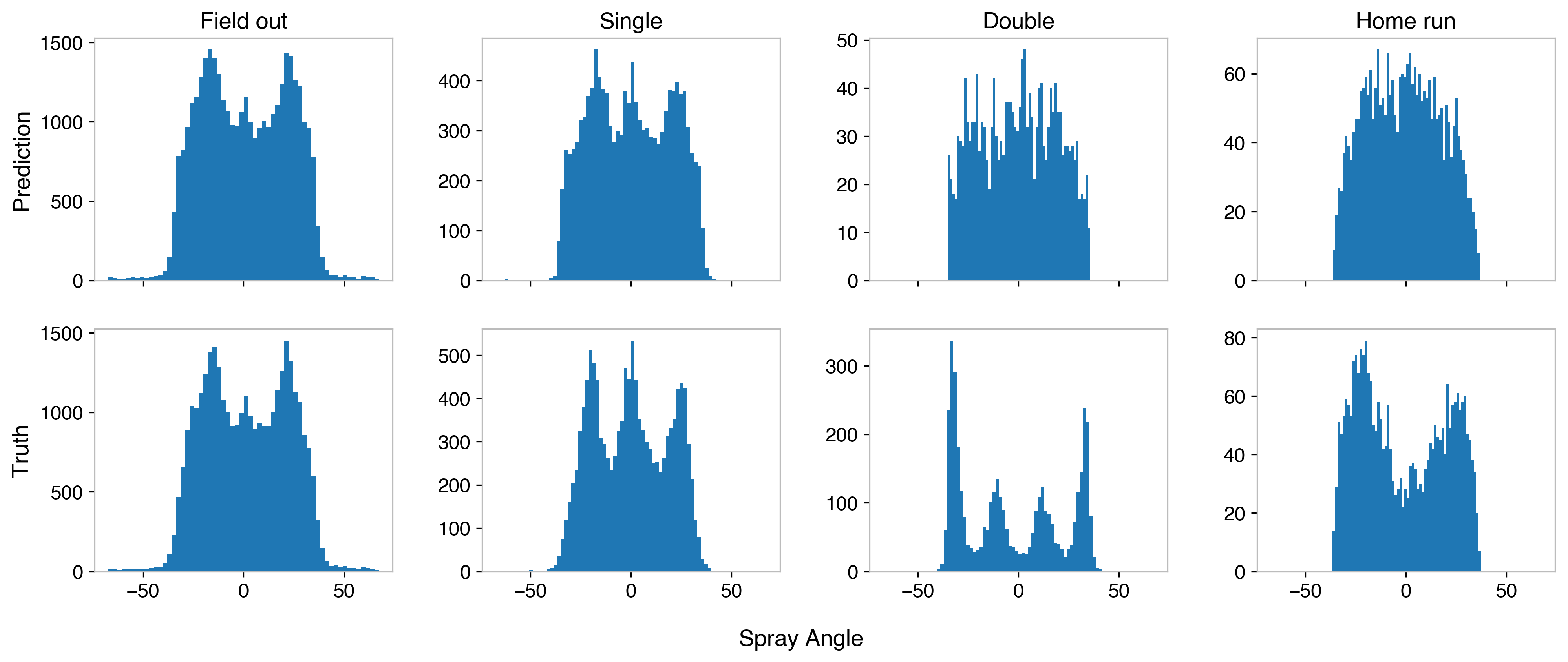
The third dimension is a very non-trivial factor though. The corners are between 300-350 ft from home, while straight-away is between 390-440 ft. First, we should take a look at how the current models are handling this (plots shown for gBDT):

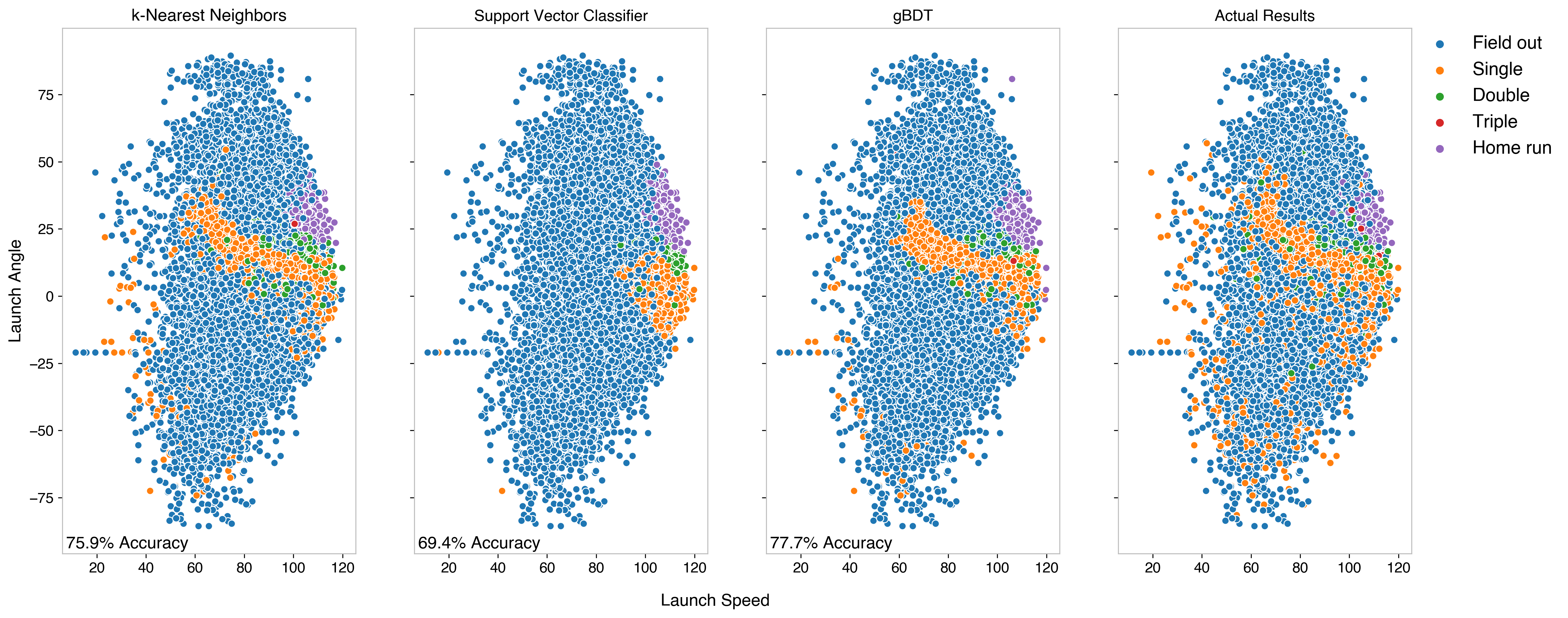
The spray angle distribution looks similar for outs and singles, but the features for doubles and home runs are not at all present. This means that adding this variable will provide the models with additional information, which should help improve the accuracy. Adding this additional variable, retraining and retesting gives the following:

Adding this variable helped out the kNN and BDT models considerably. Both increased their correct predictions on outs, singles, doubles, and home runs. Most strikingly, the prediction for doubles went from 17% accurate to 43% accurate for the BDT (24% to 49% for kNN) - this is a huge improvement. Interestingly, the SVC went from an overly liberal decision boundary on singles to an overly conservative one, which actually caused a worse overall accuracy, despite having more information.

Summary and Future Work

Ultimately, of the models tested, the best shown to classify hit outcomes based on launch angle, exit velocity, and spray angle is a BDT with a 78% accuracy. Future work on this model will focus on developing the BDT further. I’ll be following up this post with several more as I develop the BDT, which I’ll link here as they’re posted. Some topics I’m going to address:

• Acting from the “team” perspective to incorporate additional parameters (batter speed, park effects).
• Work to get the most accurate model, looking at more complex frameworks and dive into hyperparameter tuning.
• Resampling, including synthetic minority oversampling to manage imbalanced data, to assess the problem with low statistics for triples.

The code for this post can be found in this Jupyter Notebook.

Footnotes

[1] Multi-class logistic regression was also attempted, but outcomes were far worse than other models, so it was scrapped quite quickly. I also tried a Random Forest classifier in addition to the gBDT, but found the BDT to be better so elected to use it as my tree-based model. More complicated models will be addressed in future posts, but for just a few inputs, simple models are ideal.

[2] A later post will look at methods of balancing the data, by resampling methods or by expanding the sample size.

[3] Having launch angle and exit velocity allows you to break down your velocity into \(x\) (away from the batter) and \(z\) (toward the sky) components. From there, you can use the constant acceleration from gravity to derive hangtime, and then use that to evaluate distance traversed in \(x\). This is all done via physics 1 kinematic equations: first \(v_z t = - \frac{1}{2} g t^2\), where \(g\) is the acceleration of gravity (-9.8 m/s), and \(v_z\) is the \(z\) component of velocity (this ignores the height of the batter, but is close enough). Solve this for hangtime \(t\). Then plug that into \(x = v_x t\) to find the distance traversed. From a model perspective, everything else in these equations are constants, so this information is effectively encoded.

• 2023 1
• 2022 2
• 2021 1
• 2020 10
• 2019 8
• 2018 3
• 2017 1