Classifying MLB Hit Outcomes - Part 3: Studying Re-sampling Methods

Further Study at a Model to Predict Hit Outcomes

Over the last two posts, I’ve been developing a model to predict hit outcomes. In the first post, I looked at employing hit kinematics (exit velocity, launch angle, and spray angle) for this task and found that a boosted decision tree (BDT) performs best in classifying these hits. In the second post, I looked at additional features to improve accuracy, adding park effects and player speed. The domain this problem falls into is an imbalanced multiclassification problem, so I wanted to take this opportunity to look into some re-sampling methods on a real-world problem. First, though, I want to do a quick revisit in feature engineering.

Adjusted Spray Angle

I was recently reading Alan Nathan’s blog, where he posted a study on fly ball carry. I noticed that the variable used was not absolute spray angle, but an adjusted spray angle - this flips the spray angle sign (+ to - or vice versa) for left-handed batters. In doing so, the spray angle depicts push-pull angle in the x direction rather than absolute x. I wanted to take a look at if this might be more informative as a feature to my model¹. First, I plotted the distribution to see how this changes the spray angle.

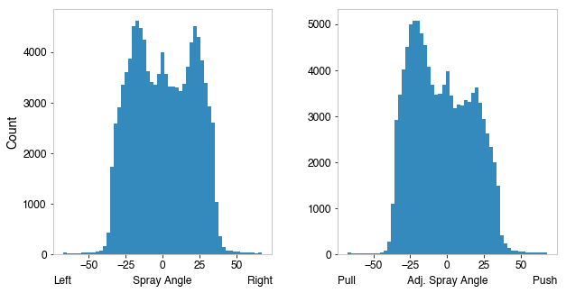
We can see the histogram becomes asymmetric, showing that pulling occurs more frequently - hopefully this is something the model can use. Next, I retrained the model, using the adjusted spray angle instead of the absolute spray angle.

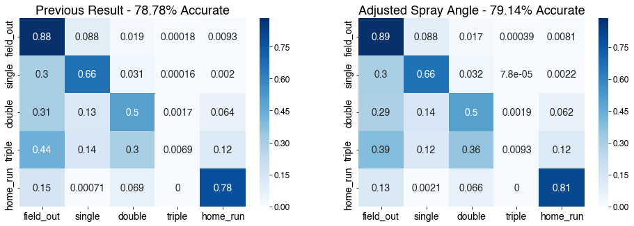
This does help improve accuracy by a bit, bringing another 0.36% accuracy gain, so I chose to keep the adjusted push/pull spray angle in my model in lieu of the absolute spray angle.

Re-sampling

Explanation and Techniques

In this section, I wanted to use this imbalanced multiclassification problem to try out and understand various re-sampling methods. To elaborate, “imbalanced” means the populations of hit outcomes are drastically different. The training data set has over 33,000 outs, which is over half of all total observations. Meanwhile, there’s only about 400 triples. Because of that imbalance, a model trained on this data will have far less opportunity to learn the parameters that result in triples, and this will affect how it makes predictions, for better or for worse.

To navigate this problem, we turn to re-sampling. Re-sampling is the method of balancing the dataset populations in the training process so each class is equally represented². For our problem, that means the training data has the same number of singles, doubles, triples, home runs, and outs. This can be achieved in two ways, upsampling and downsampling. There are several approaches to achieve either of these, for this analysis I studied 3 upsampling methods and 2 downsampling methods³.

1. Upsampling - increasing statistics in the minority classes to match the majority class

• Raw Upsampling: randomly replicating observations from your minority classes until it matches the majority population, the simplest approach to upsampling
• Synthetic Minority Oversampling Technique (SMOTE): using linear interpolation between existing points (selected via a nearest-neighbor algorithm) to create new, unique points between existing observations
• Adaptive Synthetic Sampling (ADASYN): similar to SMOTE, but focuses on generating new points in regions that are harder to learn, by generating new data in the region nearest the decision boundary

2. Downsampling - removing data from the majority classes to match the size of the minority class

• Raw Downsampling: randomly removing observations in your majority classes until they match the minority population
• NearMiss Downsampling: similar to the ADASYN focus on the decision boundaries, NearMiss uses a nearest neighbors method to isolate samples nearest the decision boundary for retention

In my experience, of the two, upsampling techniques usually work better, since in downsampling you’re getting rid of possible information the model could use (plus, nothing hurts worse than the idea of throwing away the data you worked hard to acquire and clean).

Evaluation Metric

An important note here is that when we have imbalanced datasets, one big consideration is the metric we use. The canonical example taught in binary classification is cancer screenings, in which there are few positive (“does has cancer”) cases compared to negatives (“does not have cancer”), however the cost of missing someone with cancer and leaving them untreated is much worse, so we want a model with high fidelity for the positives, even at the cost of a few extra false negatives. Another common real-world example of this is fraud flagging.

In such cases, “accuracy” is not always the best metric, so alternatives are used, such as precision, recall, or F1 score. To decide, the major question to ask is if one type of misclassification is particularly worse than another. Answering that question usually comes down to domain expertise. For this problem, my answer is no, miscategorizations for this model are all equivalently undesirable. So then I referenced a flowchart I from machinelearningmastery.com:

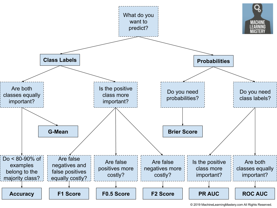
We follow the far left tree of this and stick with accuracy as our evaluation metric. This, however, gives us some assumption about what to expect from re-sampling - since the training will cause the model to learn the population ratios, and the test sample has equivalent population ratios, re-sampling likely will hurt overall performance. Nonetheless, it’s worthwhile to study, especially looking at how we can best improve the smallest minority classes.

Single Multiclassifier

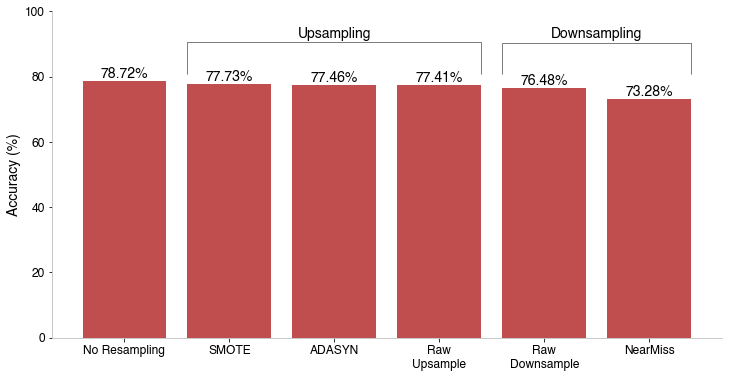
The first approach was to drop each of these techniques into the single multiclassifier with classes for each hit type, to see how each performed. To lead with the result, employing these yielded the following accuracy:

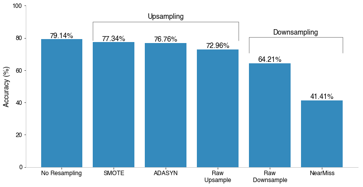
There are a few takeaways to glean from this. First, the suspicion of worse accuracy when re-sampling proved to be true, the best result was our original model without re-sampling the training data. Further, the hesitancy on downsampling specifically also was confirmed - throwing away data and re-sampling down to the minority class proved to give the worst two results. Particularly NearMiss re-sampling did over 20% worse than any other model. To understand why, I plotted the distribution of field outs for the NearMiss training data against all the training data in the launch angle/launch speed space.

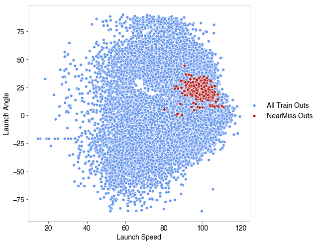
The NearMiss strategy of downsampling narrowed the range where field outs occur in this space, so it’s not trained to make predictions outside of that region. This explains the poor performance since it only predicts 28% of outs correctly.

One redeeming factor to downsampling here is that if we wanted to prioritize triple accuracy, the raw downsampled approach performed the best, accurately predicting 39% of triples, all other methods were 26% accurate or worse on triples.

Another comment is that SMOTE re-sampling performs the best of all the re-sampling. The “cleverness” in ADASYN makes it focus more around the decision boundaries. For this application, it seems to focus on the home run boundary, making it more accurate in predicting those (86% accurate for ADASYN, 84% accurate for SMOTE) at the cost of doubles (55% ADASYN vs 58% SMOTE) and triples (16% ADASYN vs 18% SMOTE).

Two-Step Classification

The next approach I wanted to analyze was a two-step classification approach. I touched on this in the appendix in the previous post, but the idea is to reframe the classification question. The single model poses the question “what is the outcome of a ball hit in play?” and tackles it with a mammoth imbalanced multiclassification problem. The two-step approach asks “is this a hit? if so, what type of hit?” This reframes the solution to a balanced binary classification problem, deciding if it is a hit, then a less imbalanced multiclassification problem, deciding what kind of hit.

In the previous appendix, I showed that, if you use the same features in both BDTs, the two-step approach does slightly worse. This might not hold true when employing re-sampling, so I revisited this idea. The approach was to do the binary classification as-is, then apply the re-sampling only on hit candidates (that is, those that passed the binary classification). The following plot shows the accuracy when applying each of the re-sampling approaches described above to just the hit candidates.

Maybe not a surprise, but the order of which re-sampling methods perform best is consistent between the two-step approach and single model approach; SMOTE still performs best. All of the resampled approaches performed better in the two-step paradigm than in the single large multiclassifier - this is because before it even reaches the multiclassifier, it starts with over 27,000 correct predictions from the binary classifier, which is 82.4% accurate on over 33,000 field outs. Even if the multiclassifier got no correct classifications, the final model would be 51% accurate due to these field outs, which is better than the single model NearMiss accuracy already.

Ultimately, since we’re considering accuracy as the figure of merit, our single model trained on imblanced data performs better than any of these, since it is trained with the expected class populations, so we’ll select that as our final model.

Summary

Wrapping up, I wanted to list some final takeaways I can gather from this post.

• Using smart features is one of the best ways to take advantage of your dataset, evidenced by the improvement by using the push/pull adjusted spray angle over the absolute spray angle.
• Re-sampling methods work most meaningfully when you have a figure of merit other than sheer accuracy, which is usually the result of a problem where a type I/II error is worse than the alternative.
• This study reinforced my already strong opinion that for most cases, you shouldn’t get rid of data if aiming for overall accuracy. The only cases I can imagine it’s useful is when you have a poorly scaling model, like an SVM, and the decision boundary is relatively well-tamed. However, if you’re very focused only on accuracy for a minority class, this can be best - the downsampled model had a 39% accuracy on triples.
• I got a lot of great experience in this using some more sophisticated re-sampling techniques, like SMOTE, ADASYN, and NearMiss. The big thing I learned is that many of them work particularly well with single decision boundaries, this is not the case for this situation. For example, there is the large band of possible singles, but there’s also plenty of possibilities for things like bunts or infield hits.

At this point, I’m satisfied with the state of this model. I’ve explored and extinguished most ideas that would improve it further. In the next and last post, I’ll discuss the utility of this model and how it can be deployed in real-world situations.

• The code for this post is contained in this Jupyter Notebook.

Footnotes

[1] To a very small degree, some of this information is embedded - when I added the park factors by handedness, this has the possibility of slightly encoding handedness, and through that, a very smart model could associate a higher tendency for certain outcomes based on that. However, that model would have to be incredibly smart to the point of overfitting, and directly coding it in is much better, as we see - it’s just possible not all the information is new, it may have been slightly represented in the older model.

[2] To emphasize - the re-sampling is performed only on the training data. Testing data is left with the standard population imbalance, because we want to understand accuracy representative of what is encountered when applying to future data.

[3] The raw re-sampling methods were performed with scikit-learn’s resample methods. All others were performed with the exceptional imbalanced-learn package.

• 2023 1
• 2022 2
• 2021 1
• 2020 10
• 2019 8
• 2018 3
• 2017 1