Nonlinear Formulas in Bambi: Gelman’s Golf Putting

☕ Buy me a coffee

Earlier this week, my PR adding support for nonlinear formulas was merged into Bambi. I’m pretty pumped about this functionality - it really expands the kinds of models that you can express through Bambi’s formula syntax.

The new functionality lets users write formulas that are nonlinear in unknown parameters, including relationships that don’t fit naturally into a conventional linear predictor. It also supports nonlinear expressions for auxiliary parameters, such as the residual standard deviation.

To show what this makes possible, I’ll walk through a few examples from the notebooks I contributed with the PR

Gelman’s Golf Putting

One of my favorite statistical modeling examples is Andrew Gelman’s golf putting case study. The goal is to model the success rate of putts given distance. He starts by putting distance into a familiar logistic regression, then improves the model by thinking about how the ball actually gets into the hole.

The original data covers putts from 2 to 20 feet. A simple binomial logistic regression models the log-odds of success as a straight line in distance. This captures declining success with distance, but doesn’t model the shape well: it overestimates success over the middle range and underestimates success on the longest putts.

Gelman instead uses a geometry-based model that considers angular error: how far can the shot stray from the intended direction and still fit into the hole? Assume the golfer aims straight at the hole, with angular errors normally distributed around zero. If the ball and hole have radii $r$ and $R$, the probability of success from distance $x$ is

\[p_{\mathrm{angle}}(x) = 2\Phi\!\left(\frac{\arcsin((R-r)/x)}{\sigma_{\mathrm{angle}}}\right)-1.\]

Here, $\Phi$ is the standard Normal cumulative distribution function, the radii and distance use the same units, and $\sigma_{\mathrm{angle}}$ is the standard deviation of angular error, measured in radians.

With this PR, we can now specify this in Bambi:

angle_formula = bmb.Formula(
    "prop(successes, attempts) ~ "
    "2 * normal_cdf(asin((hole_radius - ball_radius) / distance) / sigma_angle) - 1",
    nlpars=("sigma_angle",),
)
angle_model = bmb.Model(
    angle_formula, golf,
    family="binomial", link="identity",
    priors={"sigma_angle": bmb.Prior("HalfNormal", sigma=0.5)},
)

nlpars identifies the unknown nonlinear parameters. The expression already returns a probability, so we use an identity link. prop(successes, attempts) supplies the success and attempt counts for each distance.

Gelman’s original data: logistic regression versus the angular-error geometry model. Ribbons show uncertainty in expected success probabilities; data error bars show ±1 standard error.

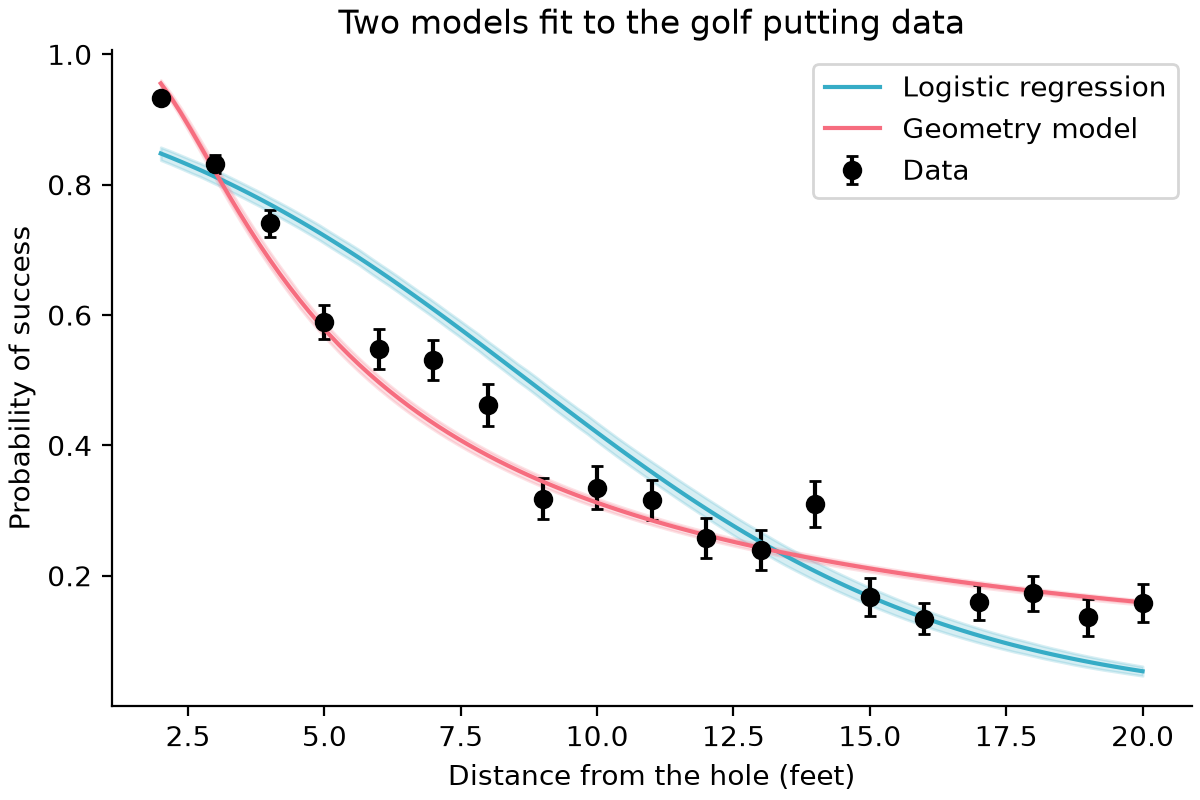
The geometry model captures the shape better. This is the type of model the PR makes possible in Bambi, putting the physical relationship directly in the formula.

Nonlinear Terms in Residual Variation

Next, Mark Broadie’s larger dataset extends to 75 feet, where the original angular model overpredicts success. This adds a distance component to our model: the ball must reach the hole without rolling too fast to fall in.

The original study assumes the golfer aims one foot past the hole. The model treats the speed as acceptable if the ball would otherwise stop between the hole and three feet beyond it. Relative to the target, that allows an error of one foot short to two feet long. Assuming Normal error with a standard deviation proportional to the intended distance, we get

\[p_{\mathrm{distance}}(x) = \Phi\!\left(\frac{2}{(x+1)\sigma_{\mathrm{distance}}}\right) -\Phi\!\left(\frac{-1}{(x+1)\sigma_{\mathrm{distance}}}\right).\]

Distances are in feet, so $x+1$ is the intended travel distance and $\sigma_{\mathrm{distance}}$ controls the relative error. Assuming independent angular and distance errors, the success probability is just their product: $\mu(x) = p_{\mathrm{angle}}(x)p_{\mathrm{distance}}(x)$.

However, there’s still variation that this physical model doesn’t capture. With so many attempts in the larger dataset, the binomial likelihood demands closer agreement than the model can provide. Gelman and Broadie account for that by approximating the observed success rates with a Normal likelihood and adding extra variance:

\[\frac{y_j}{n_j} \sim \operatorname{Normal}\!\left( \mu_j,\sqrt{\frac{\mu_j(1-\mu_j)}{n_j}+\sigma_y^2} \right).\]

In the variance, the first term inside the square root, $\mu_j(1-\mu_j)/n_j$, captures the variation we’d expect from a finite number of attempts. The extra term, $\sigma_y^2$, accounts for variation the physical model doesn’t capture. This is a nice feature of the new nonlinear API: the residual standard deviation can be a nonlinear function of the mean and other unknown parameters.

In Bambi, we can name the two probability expressions and combine them:

angle_probability_expression = (
    "2 * normal_cdf(asin((hole_radius - ball_radius) / distance) / sigma_angle) - 1"
)
distance_probability_expression = (
    "normal_cdf(2 / ((distance + 1) * sigma_distance)) - "
    "normal_cdf(-1 / ((distance + 1) * sigma_distance))"
)

golf_residual_formula = bmb.Formula(
    "success_rate ~ p_angle * p_distance",
    f"p_angle ~ {angle_probability_expression}",
    f"p_distance ~ {distance_probability_expression}",
    "sigma ~ 0.5 * log(mu * (1 - mu) / attempts + sigma_y ** 2)",
    nlpars=("p_angle", "p_distance", "sigma_angle", "sigma_distance", "sigma_y"),
)

Here, mu is the mean success probability, p_angle * p_distance. For a Gaussian model, Bambi uses a log link for sigma by default, so its formula specifies half the log variance. Applying the inverse link gives the square root in the equation above.

Model with residual variation. Lower bands are fitted conditional ±1σ and ±2σ scales.

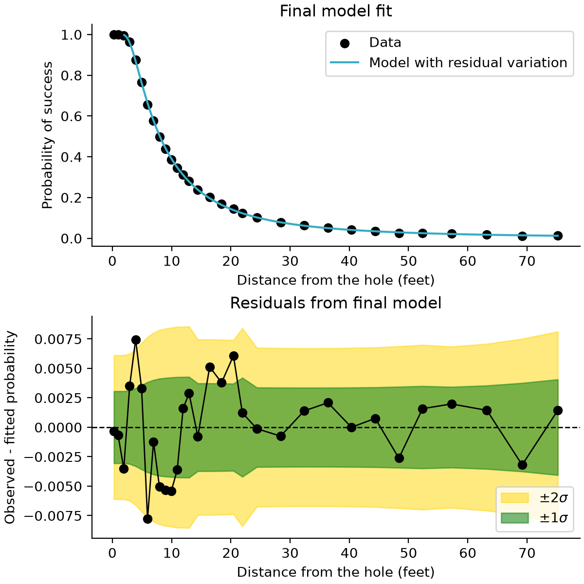
The fitted curve follows the data closely, with small residuals in the lower panel. Most fall within the wider $2\sigma$ band.

These are highlights from the case study. I reconstructed the full model-building sequence in the golf notebook, which will join Bambi’s example gallery with the next release.

Beyond golf

My companion notebook looks at two other uses with classic datasets included in R: Puromycin for enzyme kinetics and Orange for tree growth.

Enzyme kinetics

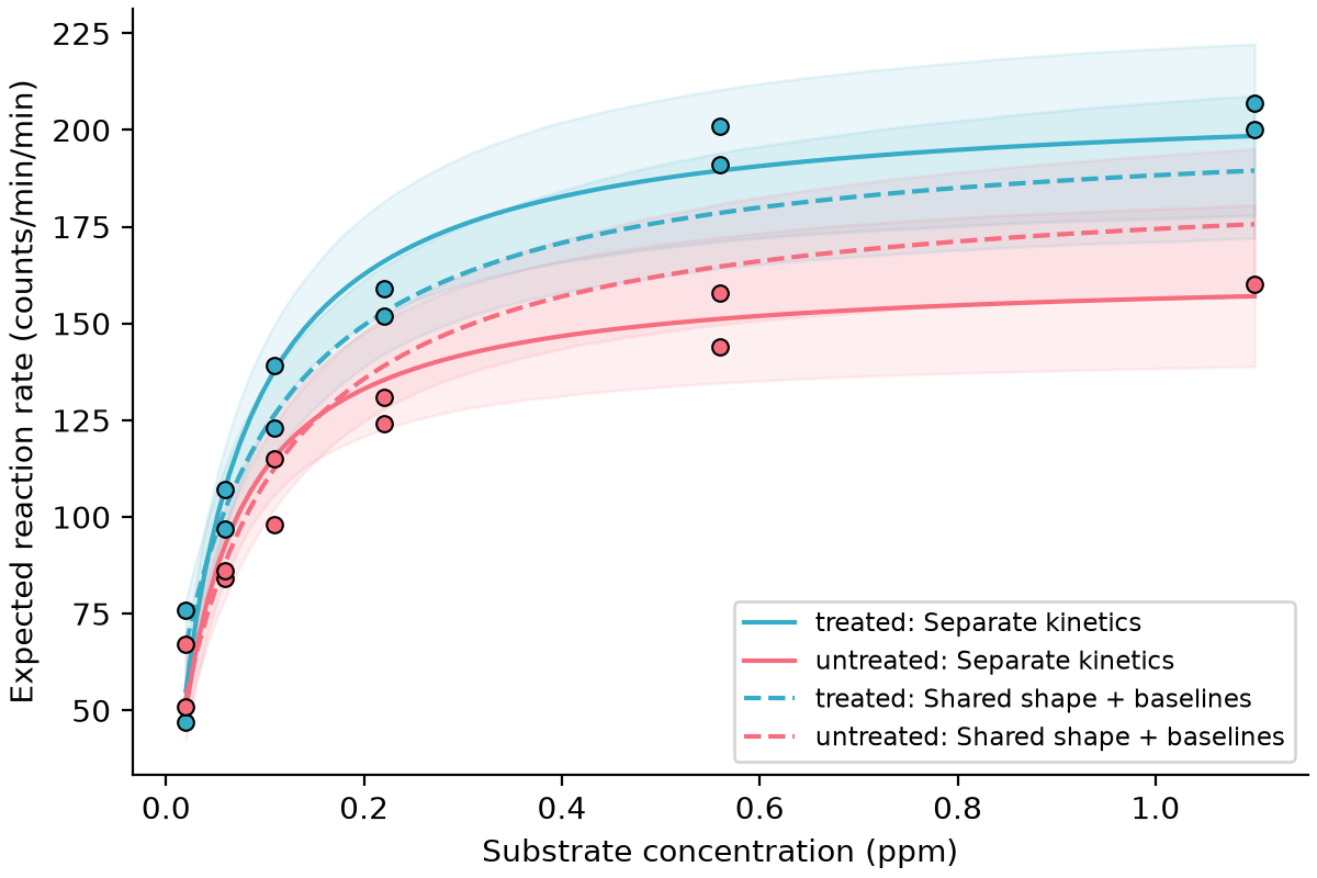
The Puromycin data contains reaction rates at different substrate concentrations for treated and untreated cells. The Michaelis–Menten curve describes the expected rate at concentration $c_i$:

\[\mu_i = \frac{V_{\max,i}c_i}{K_{m,i}+c_i}.\]

$V_{\max}$ is the maximum rate the curve approaches, and $K_m$ is the concentration at half that rate. We can let both parameters differ by treatment in Bambi:

mm_formula = bmb.Formula(
    "rate ~ vmax * concentration / (km + concentration)",
    "vmax ~ 0 + state",
    "km ~ 0 + state",
    nlpars=("vmax", "km"),
)

Here, state identifies the treatment, and 0 + state gives each treatment its own coefficient. Alternatively, we can share the curve and let treatment shift the baseline:

\[\mu_i = \beta_{\mathrm{state}[i]} + \frac{V_{\max}c_i}{K_m+c_i}.\]

mixed_formula = bmb.Formula(
    "rate ~ 0 + nl(vmax * concentration / (km + concentration)) + state",
    nlpars=("vmax", "km"),
)

nl(...) adds the nonlinear curve directly to the mean, without an extra coefficient. Outside it, 0 + state gives each treatment its own baseline. In this version, each curve approaches its baseline plus $V_{\max}$.

Both models use a Gamma likelihood with an identity link and positive priors. They produce the following curves:

Puromycin: separate treatment kinetics versus a shared curve with additive baselines. Shading shows 94% equal-tailed intervals for expected rates.

Tree growth

The Orange data follows the trunk circumference of five trees over time. We can describe growth with a logistic curve:

\[y_{ij} = \frac{A_j}{1+\exp((x_{\mathrm{mid}}-x_{ij})/s)} + \epsilon_{ij}, \qquad \epsilon_{ij} \sim \operatorname{Normal}(0,\sigma).\]

Here, $A_j$ is tree $j$’s eventual trunk circumference in the model, $x_{\mathrm{mid}}$ is the age when it reaches half that size, and $s$ determines how quickly it grows. In Bambi, this looks like:

orange_formula = bmb.Formula(
    "circumference ~ asym / (1 + exp((xmid - age) / scale))",
    "asym ~ 1 + (1 | tree)",
    nlpars=("asym", "xmid", "scale"),
)

Orange trees: partially pooled tree-specific asymptotes, with uncertainty in mean growth curves rather than individual measurements.

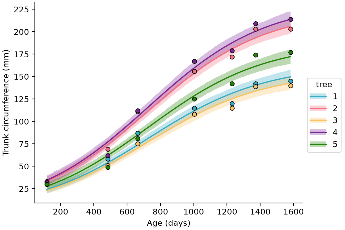
asym ~ 1 + (1 | tree) lets each tree have its own asymptotic circumference while borrowing information across trees. The growth midpoint and timescale stay shared.

Wrapping Up

What I like about these examples is that we can build models that more closely reflect how the data are generated, with parameters that describe something concrete: angular accuracy, reaction kinetics, or tree size. We can write those relationships directly while keeping Bambi’s familiar formula syntax for treatment effects and differences between groups.

This functionality is now in the dev branch and will be available in the next release. Thanks to Tomas Capretto for his feedback and help getting this work over the line.