Forecasting March Madness 2026 - Latent Skills Models

For live updates throughout the tournament, see the dashboard.

Background

Every March, 68 college basketball teams from 31 conferences get thrown into a single-elimination bracket, and \(2^{63}\) (roughly 9.2 quintillion) possible outcomes follow. I find bracketology to be a really fun statistical problem: individual games are often fairly predictable, but with that many possible outcomes, low-probability upsets are virtually guaranteed to sneak through somewhere. Everyone’s bracket breaks. That’s why even an octopus can put together competitive predictions for single-elimination tournaments.

For this year’s tournament, I fit a model to forecast the NCAA March Madness tournaments. The approach builds on the same philosophy as my NHL team strength model, a hierarchical Bayesian model for handling head-to-head matchups where we have historical scores. This model decomposes team quality into attack and defense parameters, and the same decomposition is a natural fit for basketball. By decomposing offense and defense, we can see how Houston’s defense-first approach is fundamentally different from Alabama’s strong offensive profile. Simulating bracket knowing how a team wins, not just that it wins provides a richer, more digestible understanding of the predictions.

The Model

Step 1: Bradley-Terry (Win/Loss)

The classic Bradley-Terry model assigns each team \(i\) a latent strength \(\theta_i\) and models the probability that team \(i\) beats team \(j\) as a function of the difference in their strengths. In its typical form, the only outcome is binary: who won. This is a workhorse model for pairwise comparisons (Elo ratings are a special case) and it works fine for generating bracket probabilities.

But basketball gives us more than just wins and losses. Beating a team by 30 tells you something very different than winning by 1, but the basic Bradley-Terry model sees those as equivalent.

Step 2: Score Differential

A natural extension is to model the score margin directly:

\[\text{margin}_{ij} \sim \text{Normal}(\theta_i - \theta_j + \alpha \cdot \text{home}_i, \sigma)\]

Now \(\theta_i\) captures how many points team \(i\) is above or below average, and the likelihood uses the full margin rather than collapsing it to a binary outcome. Home court advantage \(\alpha\) enters linearly. I stood this up initially, and it achieved a Brier score of 0.189 across 10 seasons of held-out tournament predictions.

But this model still assigns each team a single “strength” number. Michigan and Houston might have the same \(\theta\), but they get there in completely different ways. The single strength parameter can’t see that.

Step 3: Offense-Defense Decomposition

In this approach, each game produces two observations, the score produced by each team. By observing each team’s score separately, you can naturally split team strength into offense and defense:

\[\text{score}_i \sim \text{Normal}(\mu + \text{off}_i - \text{def}_j + \alpha \cdot \text{home}_i, \sigma)\] \[\text{score}_j \sim \text{Normal}(\mu + \text{off}_j - \text{def}_i - \alpha \cdot \text{home}_i, \sigma)\]

Each team gets two parameters: an offensive strength \(\text{off}_i\) (how many points they generate above average) and a defensive strength \(\text{def}_i\) (how many points they prevent above average). The global intercept \(\mu\) anchors the average score per team per game, estimating at about 70 points. Home court advantage \(\alpha\) applies in the usual way.

Note that if you subtract the second equation from the first, you recover the margin model. Any information the margin model could learn, this model can as well. What it gains is the ability to distinguish Houston’s defense-first 77-55 wins from Michigan’s offense-first 101-83 wins, even when both are comfortable victories.

This is the same framework Baio & Blangiardo used for modeling the Premier League, adapted for college basketball. The key insight from that work carries over: by modeling scores directly instead of margins, you can identify teams that win by outscoring opponents versus teams that win by shutting them down.

Hierarchical Structure and the LKJ Correlation

Not all teams are created equal in terms of schedule strength. A mid-major team that went 28-3 against weak competition: how good are they really? I handle this with a hierarchical prior. Each team’s offense and defense are drawn from conference-level distributions:

\[\begin{bmatrix} \text{off}_i \\ \text{def}_i \end{bmatrix} = \begin{bmatrix} \mu^{\text{off}}_{c[i]} \\ \mu^{\text{def}}_{c[i]} \end{bmatrix} + L \cdot z_i\]

where \(L\) is the Cholesky factor of a \(2 \times 2\) covariance matrix with an LKJ(\(\eta=2\)) prior on the correlation, and \(z_i \sim \text{Normal}(0, 1)\). Conference-level means for offense (\(\mu^{\text{off}}_c\)) and defense (\(\mu^{\text{def}}_c\)) are estimated separately. The SEC might produce strong defenses while the Big Ten generates potent offenses, or vice versa.

The LKJ prior lets the model learn whether offense and defense trade off or co-occur within a conference. The non-centered parameterization via \(z_i\) is the standard trick for sampling efficiency in hierarchical models.

The ultimate result is that we get conference-level effects: a dominant team in a weak conference gets pulled down slightly, and an underperforming team in a strong conference gets a boost.

On the likelihood

One decision to make in this process is the likelihood for number of points scored in a game. Here we balance pragmatism and expressiveness.

In basketball, points are discrete units so a natural question is why not use a Poisson or negative binomial likelihood? A couple of reasons:

• Basketball scores are sums of 1/2/3-point possessions, not a genuine counting process. A team’s score of 78 isn’t “78 events occurred” the way 3 goals in a hockey game is.
• At a mean of ~70 points, the Gaussian puts essentially zero mass below zero, and by the central limit theorem it’s a good approximation to a sum of many small discrete contributions anyway.
• The continuous approximation (Gaussian) is simpler and easier to fit, which was helpful given I had one night to put this together.

With individual scores instead of margins, outliers become a concern. Blowout games could pull the model around. To handle this empirically, I fit both a Gaussian and a Student-t likelihood (which is more robust to outliers) and compared them via LOO cross-validation:

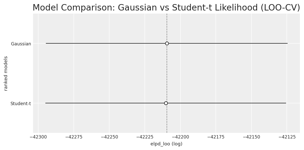
The ELPD difference was negligible in favor of Gaussian. The Student-t model estimated \(\nu \approx 53\), which is basically indistinguishable from a Gaussian, so I kept the Gaussian for simplicity.

Full Model Specification

with pm.Model(coords=coords) as model:
    mu_intercept = pm.Normal("mu_intercept", mu=70, sigma=10)

    sigma_off_conf = pm.HalfNormal("sigma_off_conf", sigma=5)
    sigma_def_conf = pm.HalfNormal("sigma_def_conf", sigma=5)
    mu_off_conf = pm.Normal("mu_off_conf", mu=0, sigma=sigma_off_conf, dims="conference")
    mu_def_conf = pm.Normal("mu_def_conf", mu=0, sigma=sigma_def_conf, dims="conference")

    sd_dist = pm.HalfNormal.dist(sigma=5)
    chol, corr, stds = pm.LKJCholeskyCov("lkj", n=2, eta=2, sd_dist=sd_dist,
                                          compute_corr=True)
    z = pm.Normal("z", mu=0, sigma=1, shape=(n_teams, 2))

    team_effects = pt.stack([mu_off_conf[conf_of_team],
                             mu_def_conf[conf_of_team]], axis=1) + pt.dot(z, chol.T)
    off = pm.Deterministic("off", team_effects[:, 0], dims="team")
    deff = pm.Deterministic("def", team_effects[:, 1], dims="team")

    alpha = pm.Normal("alpha", mu=3.5, sigma=2.0)
    sigma = pm.HalfNormal("sigma", sigma=15)

    mu_score_i = mu_intercept + off[team_i] - deff[team_j] + alpha * home
    mu_score_j = mu_intercept + off[team_j] - deff[team_i] - alpha * home

    pm.Normal("score_i", mu=mu_score_i, sigma=sigma, observed=score_i, dims="game")
    pm.Normal("score_j", mu=mu_score_j, sigma=sigma, observed=score_j, dims="game")

Sampled with nutpie: 4 chains, 2,000 draws each after 2,000 tuning steps. Zero divergences, \(\hat{R} \leq 1.01\) for all parameters.

Data

The model is fit on the 2025-26 regular season: all 5,647 Division I games across 365 teams and 31 conferences. Data comes from the Kaggle March ML Mania 2026 competition dataset. Each game provides: which teams played, both scores, and whether it was a home game, away game, or neutral site.

Posterior Predictive Check

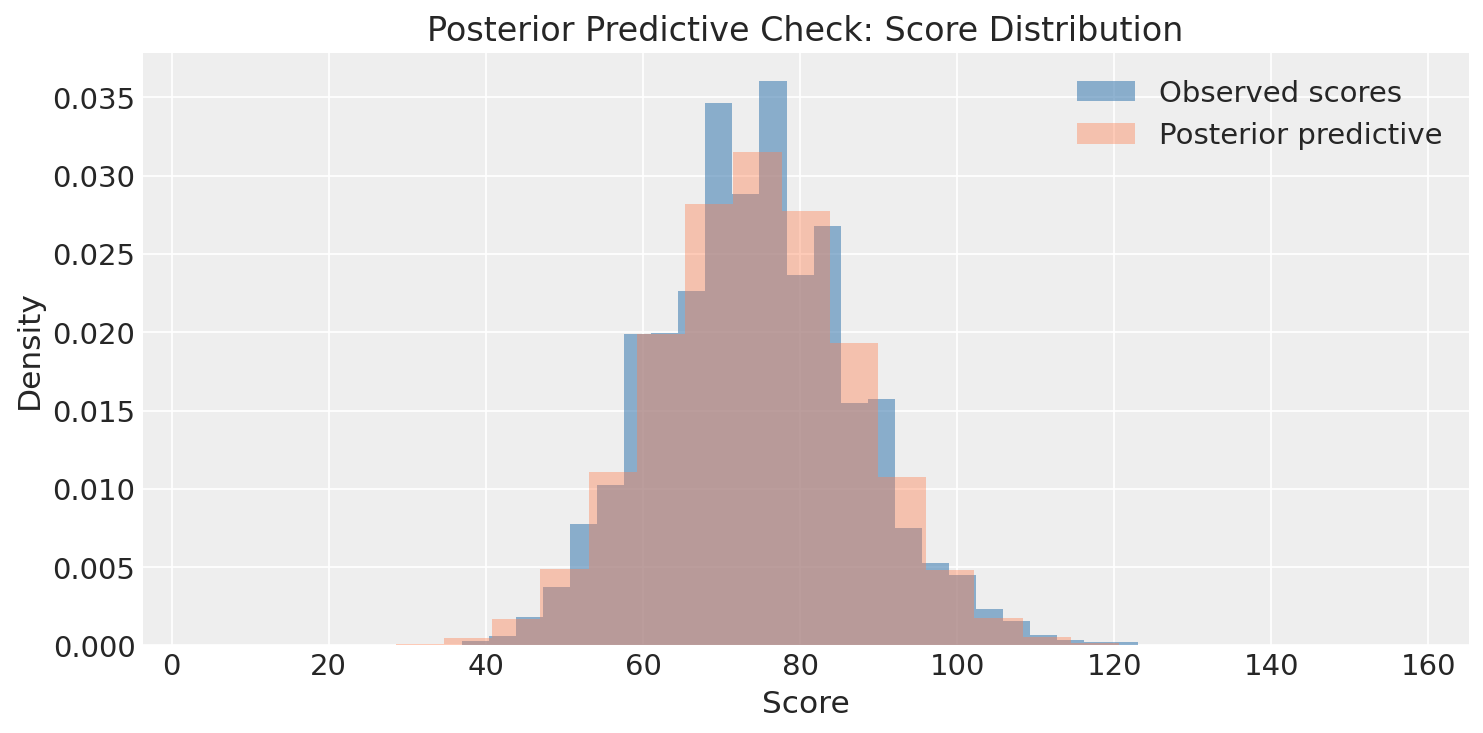
The posterior predictive distribution matches the observed score distribution well.

Results

Overall Team Strength

The overall strength of a team is the sum of its offensive and defensive contributions: \(\text{off}_i + \text{def}_i\).

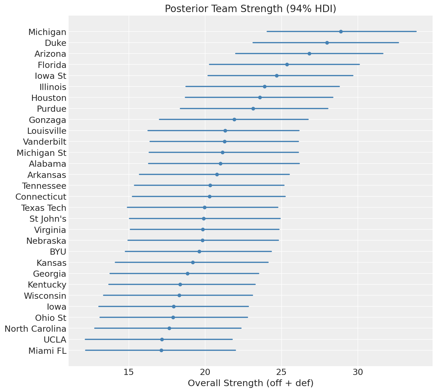
Michigan and Duke sit at the top, followed by Arizona and Florida. These are the 4 number one seeds. Some may say this is chalky, I say it’s a great sanity check.

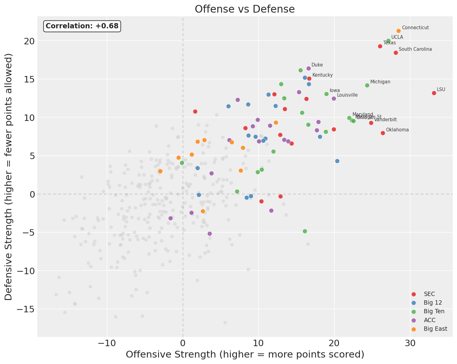
The Offense-Defense Decomposition

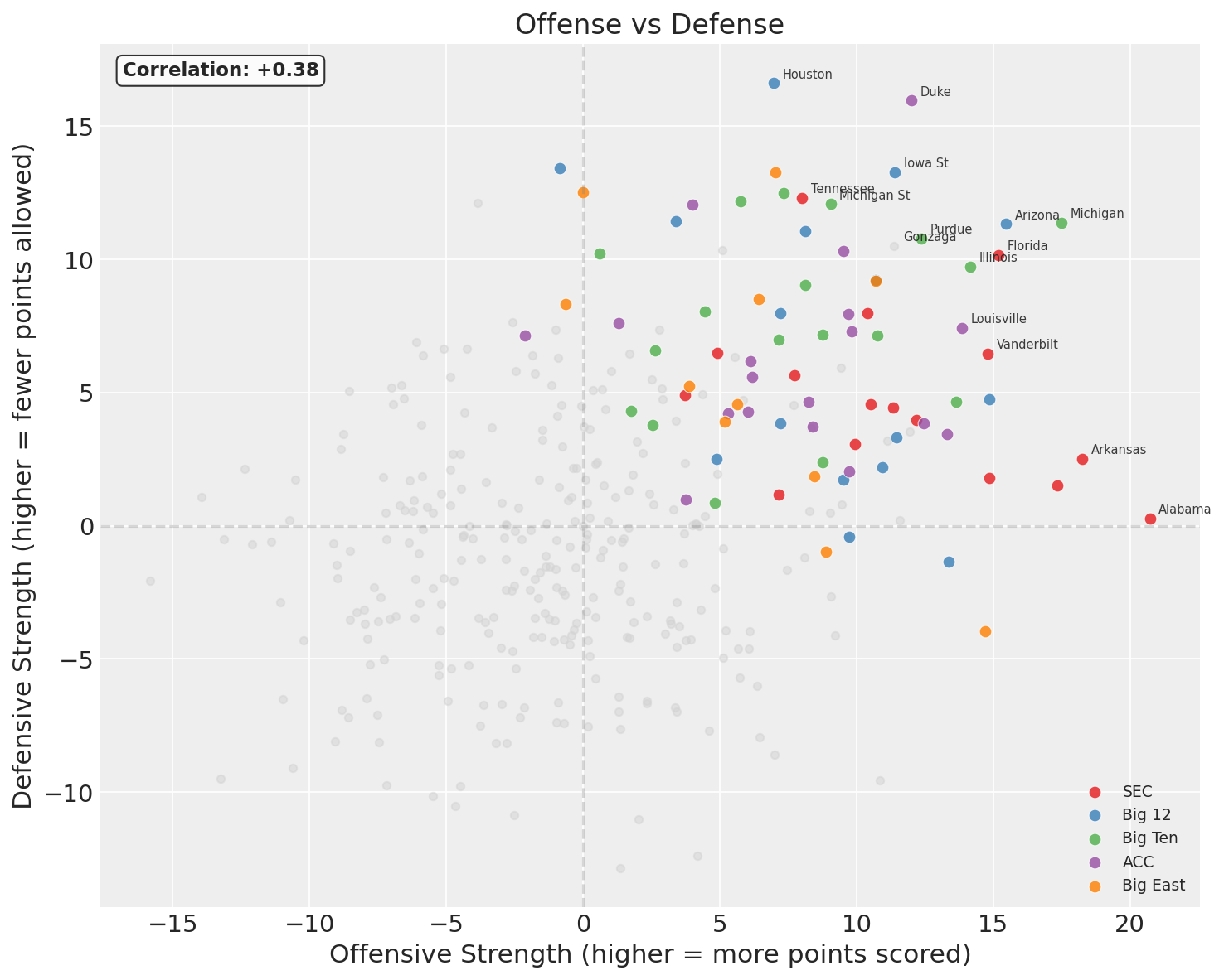
Every dot is a team, grey ones are those that didn’t make the tournament. The x-axis is offensive strength (higher = generates more points above average), the y-axis is defensive strength (higher = allows fewer points than average). Teams in the upper-right are good at both; teams in the lower-left are bad at both.

A few teams to highlight:

• Houston (overall 23.6): off = 7.0, def = 16.6. This is a defense-first team by a wide margin. Elite defensive rating, merely decent offense.
• Alabama (overall 21.0): off = 20.7, def = 0.3. The highest offensive rating of any tournament team, however paired with defense essentially at the league average.
• Duke (overall 28.0): off = 12.0, def = 16.0. Also defense-first, but with a more balanced profile than Houston.

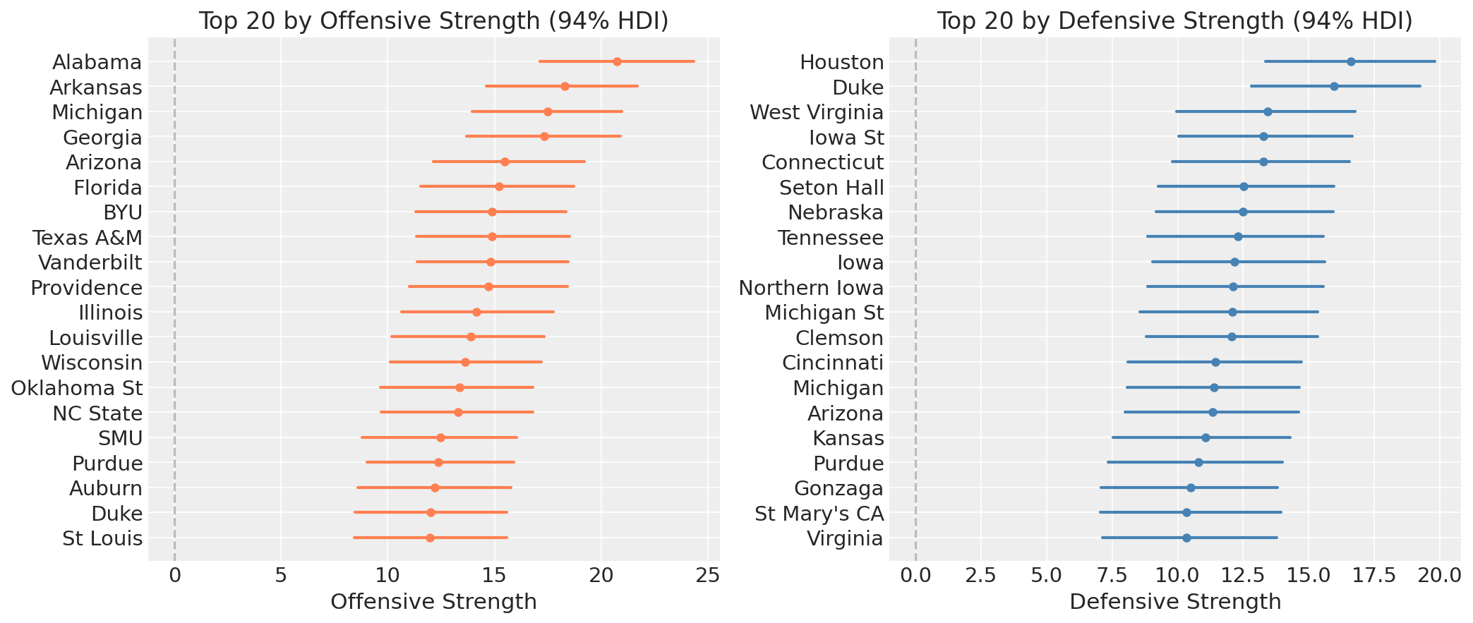
The side-by-side rankings make the decomposition concrete. The list of top-20 offenses and top-20 defenses are quite different. A team can rank in the top 5 offensively while barely cracking the top 20 defensively, or vice versa.

Physically, \(\text{off}_i\) is how many points above average team \(i\) produces per game, and \(\text{def}_i\) is how many points below average they hold opponents to. These are per-game quantities, not per-possession, so they bake in pace alongside efficiency.

Conference Effects: Offense vs Defense

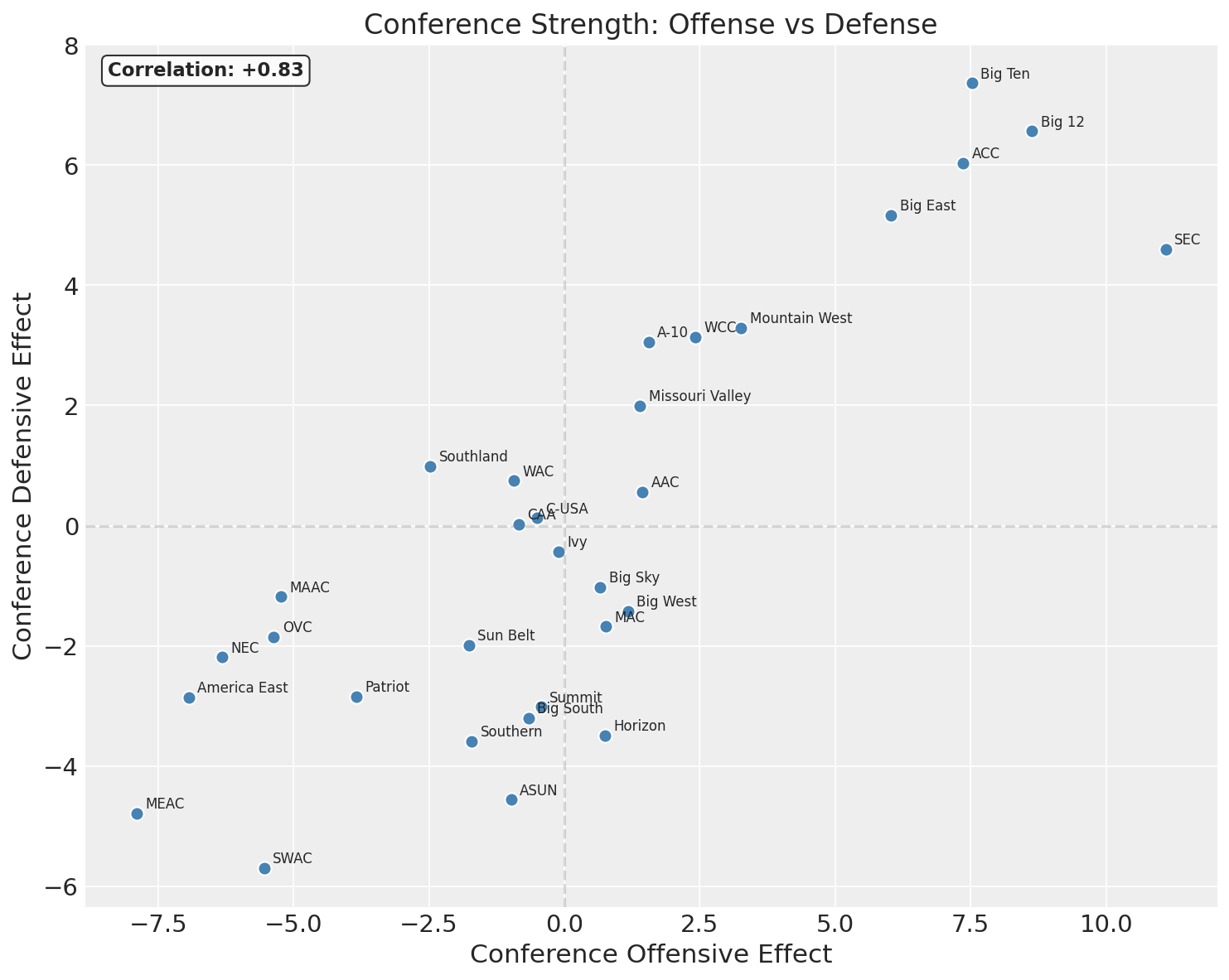
Conferences generally don’t lean dramatically in one direction or the other - good conferences are good, bad conferences are bad. The correlation in offensive and defensive effects is 0.83, very strong.

Shooters Shoot - Simpson’s Paradox in the Wild

One thing worth noting in the plot above is the marginal correlation between offense and defense across all 365 teams is +0.38. That’s positive: teams that are good at offense tend to also be good at defense. Intuitively, this makes sense: programs with good coaching, recruiting, and resources tend to be good at everything.

But the LKJ model parameter, the within-conference correlation that the model learned, is -0.20. That’s negative. Within a conference, offense and defense trade off. This is Simpson’s paradox. The relationship reverses when you condition on the confounding variable (conference membership). Here’s why:

Between conferences, the correlation is +0.83. Strong conferences (SEC, Big 12, Big Ten) produce teams that are above average on both offense and defense. Weak conferences produce teams below average on both. This between-group correlation is strong and positive, and when you pool all teams together ignoring conference, it dominates the marginal relationship.

Within a conference, though, there’s also a structural component: games are zero-sum at the score level. When Team A runs up the score on Team B, that same game hurts Team B’s defensive numbers. One team’s strong offensive showing is simultaneously a poor defensive showing for the opponent, and conference opponents play each other repeatedly, effectively inducing a negative correlation. The data suggests a modest negative correlation of about -0.20 within conferences, largely shaking out from this.

The LKJ model parameter of -0.20 captures precisely this within-conference structure. That’s what it’s designed to do: after the conference means (\(\mu^{\text{off}}_c\), \(\mu^{\text{def}}_c\)) absorb the between-conference variation, the LKJ correlation models the residual relationship between offense and defense at the team level.

Home Court Advantage

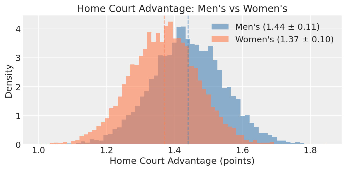
The model estimates \(\alpha\) at 1.44 ± 0.11 points. At first glance this looks low, but remember that \(\alpha\) appears in both score equations with opposite signs: the home team’s expected score goes up by \(\alpha\), and the away team’s goes down by \(\alpha\). The net effect on the margin is \(2\alpha \approx 2.9\) points, consistent with the published literature and KenPom’s estimate of ~3.5 raw points (our estimate is slightly lower because the model accounts for team quality differences simultaneously).

This parameter matters for training but zeroes out for tournament predictions, since all men’s tournament games are on neutral courts. I’ll come back to why this distinction matters for the women’s tournament later.

Simulating the Tournament

Win probabilities come from the Gaussian CDF applied to the strength difference. For two teams \(i\) and \(j\) on a neutral court:

\[P(i \text{ beats } j) = \Phi\left(\frac{(\text{off}_i - \text{def}_j) - (\text{off}_j - \text{def}_i)}{\sigma\sqrt{2}}\right)\]

The \(\sqrt{2}\) comes from the fact that we’re comparing the difference of two independent score random variables, each with variance \(\sigma^2\).

For each of 10,000 simulations, I draw a complete set of team strengths from the posterior and play through the 68-team bracket. If only I could spam all of them to my bracket pool.

Championship Odds

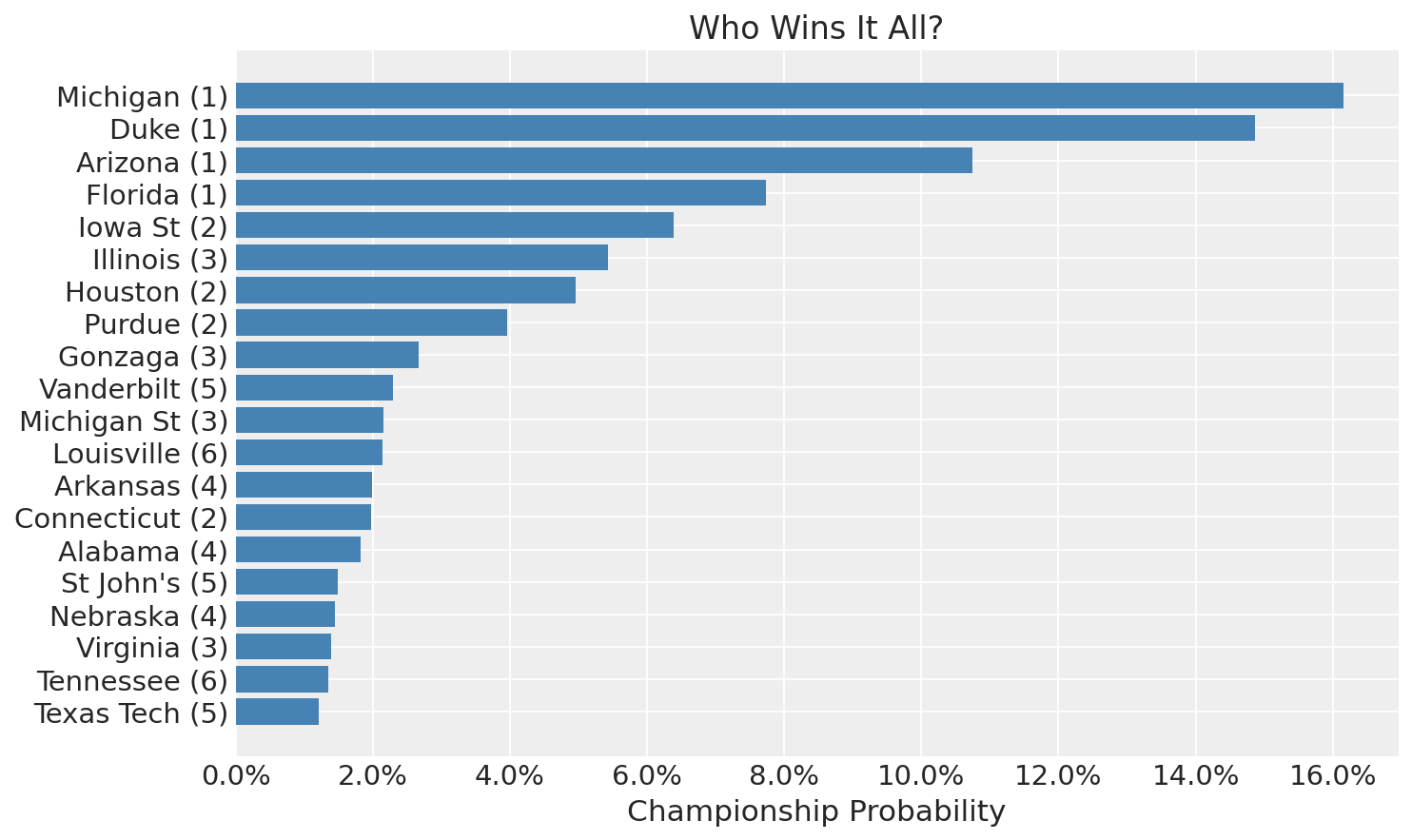
Again, the four number one seeds rise to the top, monopolizing nearly 50% of the championship probability. However, that does mean a 50% chance none of them win the tournament.

Advancement Probabilities

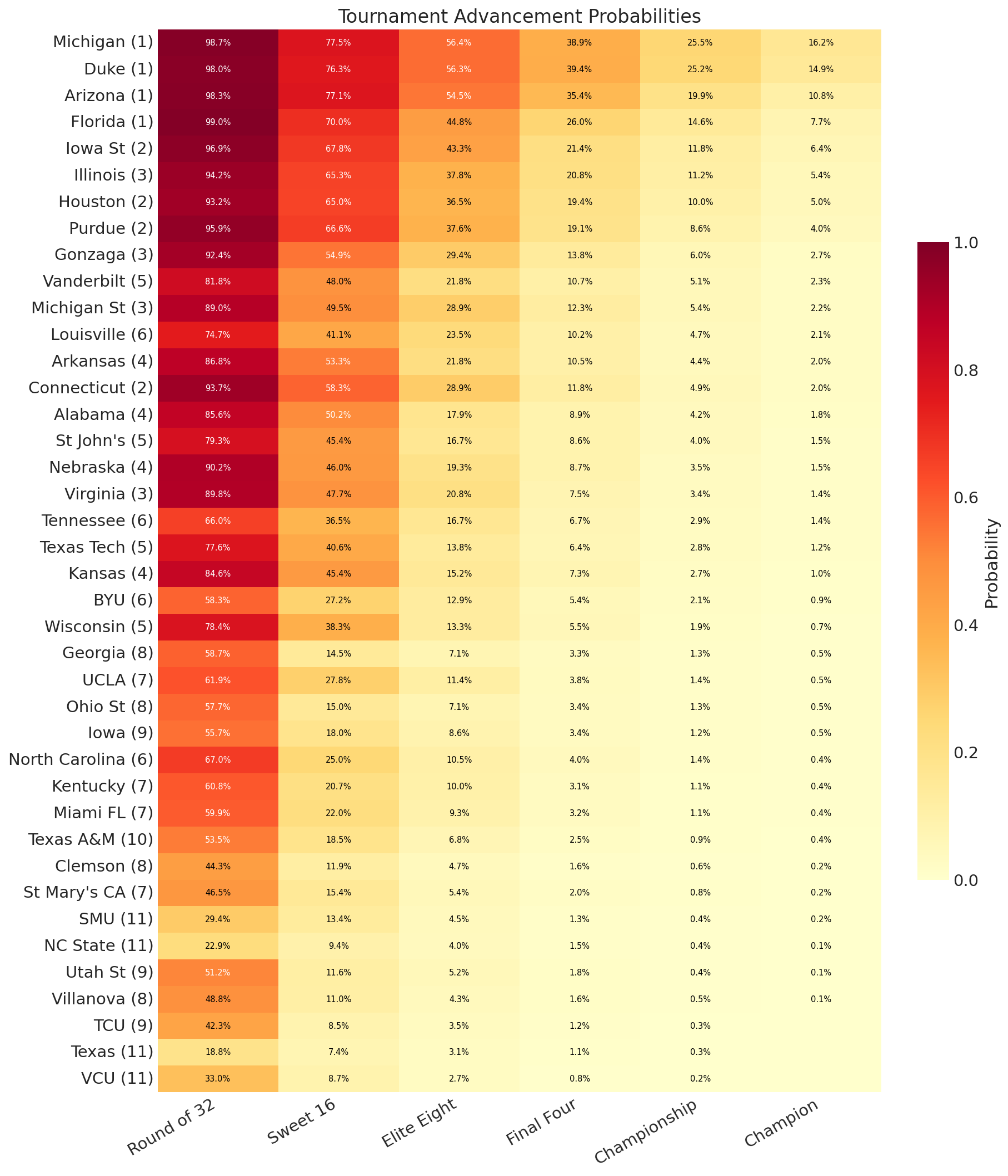
The advancement heatmap tells the full story. Notice how probability drops off dramatically at each round. Even #1 seeds only have ~50% probability of making the Final Four. This is because as the tournament progresses, you’re playing better competition, and you have more and more hurdles to clear. If the first round you have a 10% chance of dropping, the second you have 20%, that’s a total of a 28% chance of dropping out in the first two rounds, worse than one-in-four.

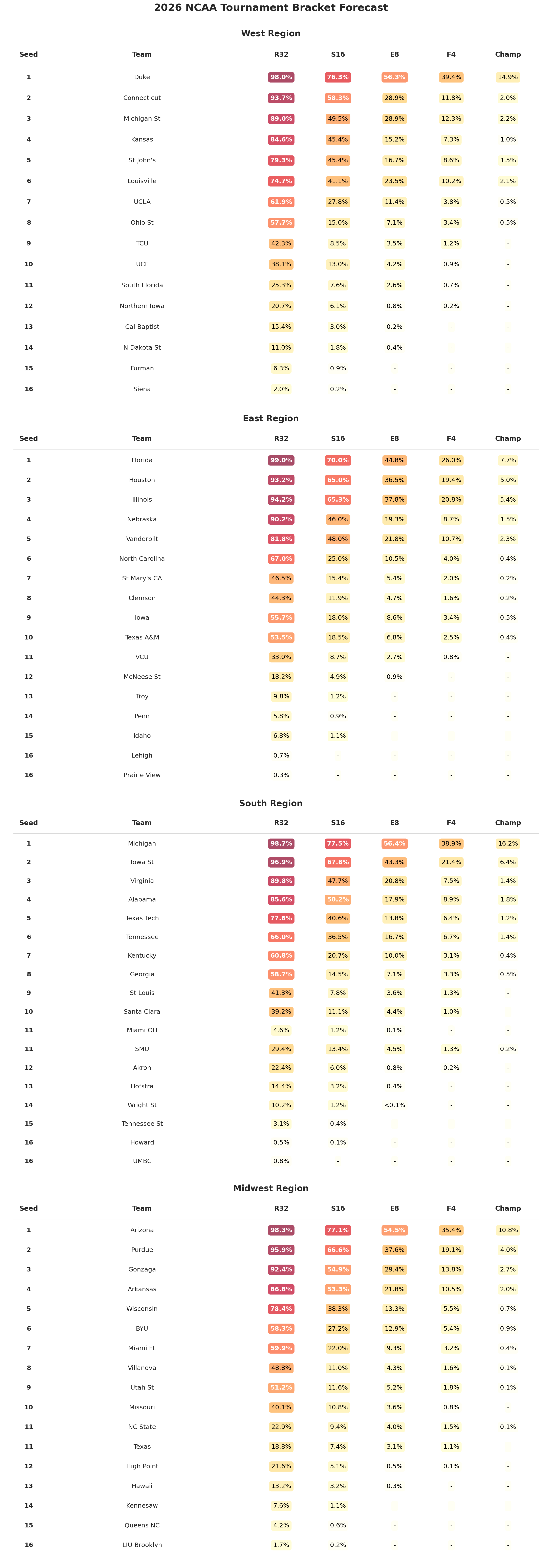
Below is the breakdown by region:

Upset Watch

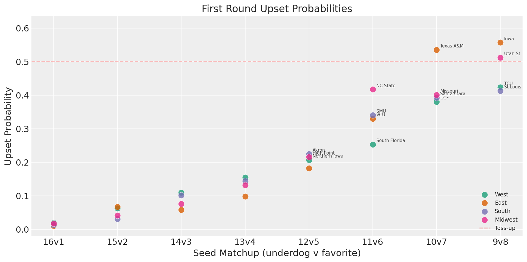
Worth noting that the model is fairly chalky here. It will generally agree with the committee’s seeding, since it’s estimating overall team strength from the same regular season data. However, it does see Texas A&M as the one 10 seed to beat a 7 in the first round (though, it’s just over 50%, so effectively a coin flip).

Tail Outcomes

The most fun part of running 10,000 brackets: the tail outcomes. These are things that could happen, the model assigns them nonzero probability, even if they’re unlikely.

Deepest Cinderella runs across 10,000 simulations:

• Northern Iowa (12) won the championship in 2 simulations
• NC State (11) and SMU (11) each won the championship
• Cal Baptist (13) reached the Championship game
• Tennessee St (15) reached the Championship game
• Siena (16) reached the Elite Eight

Historical Validation

I validated by fitting the offense-defense model on each regular season from 2015–2025 (skipping 2020’s COVID cancellation) and predicting that year’s tournament.

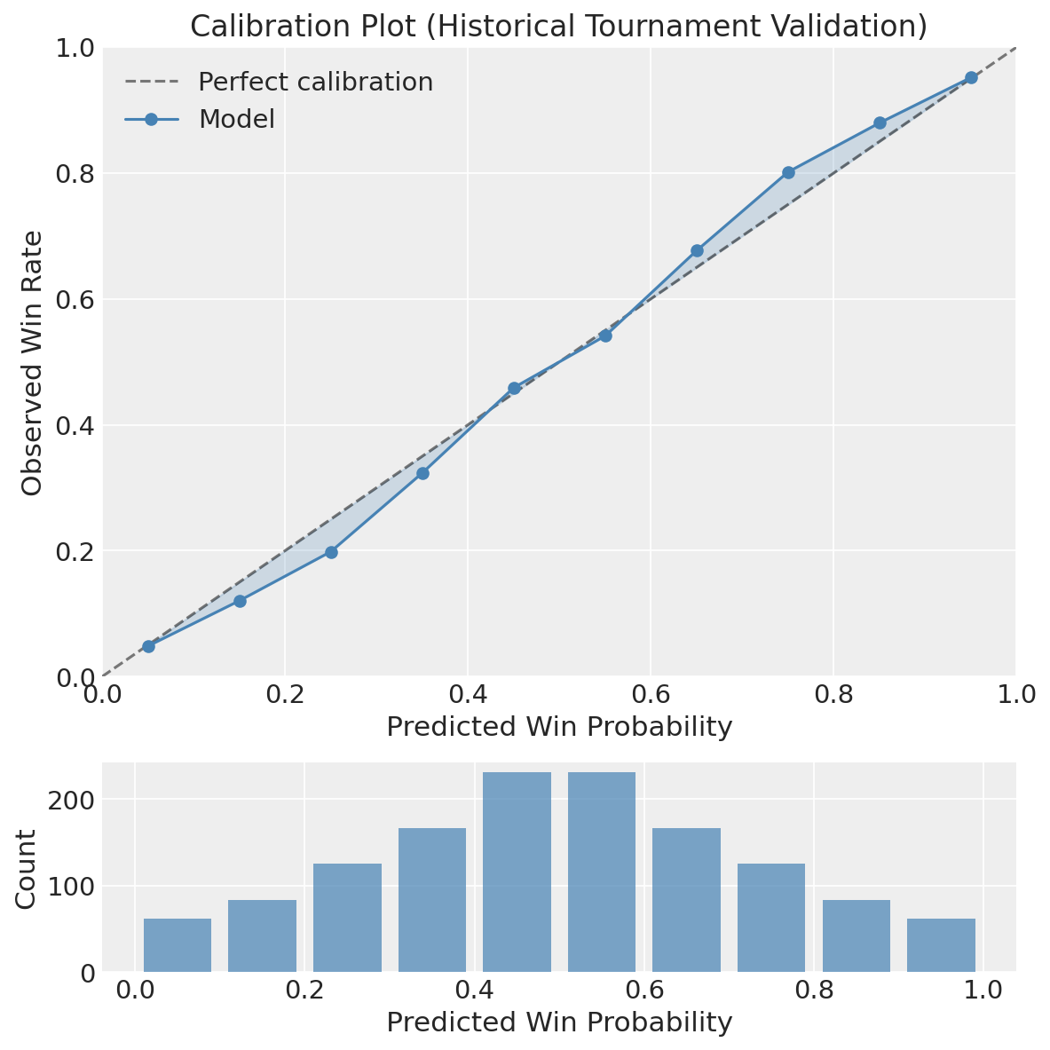
Results across 669 tournament games:

• Brier score: 0.189
• Accuracy: 70.4%
• Log loss: 0.555

It is worth calling out that this Brier score is equivalent to a single strength parameter model. Sort of a no-free-lunch thing going on here, we’re a bit constrained by using just the score margin as our outcome. That being said, the decomposition paints a much clearer picture of team structure, making the model interpretable and useful in a way not achievable by a single parameter model.

The calibration plot shows the model is reasonably well-calibrated. There is a slight bit of the characteristic “s-curve” shape which comes from overfitting that could be improved upon in the future.

The Women’s Tournament

I fit an independent model on the women’s regular season using the identical offense-defense specification. The results tell a very different story from the men’s tournament.

UConn and the Chalkiness Gap

The men’s tournament has two co-favorites separated by 1.3 percentage points. The women’s tournament has UConn and everyone else:

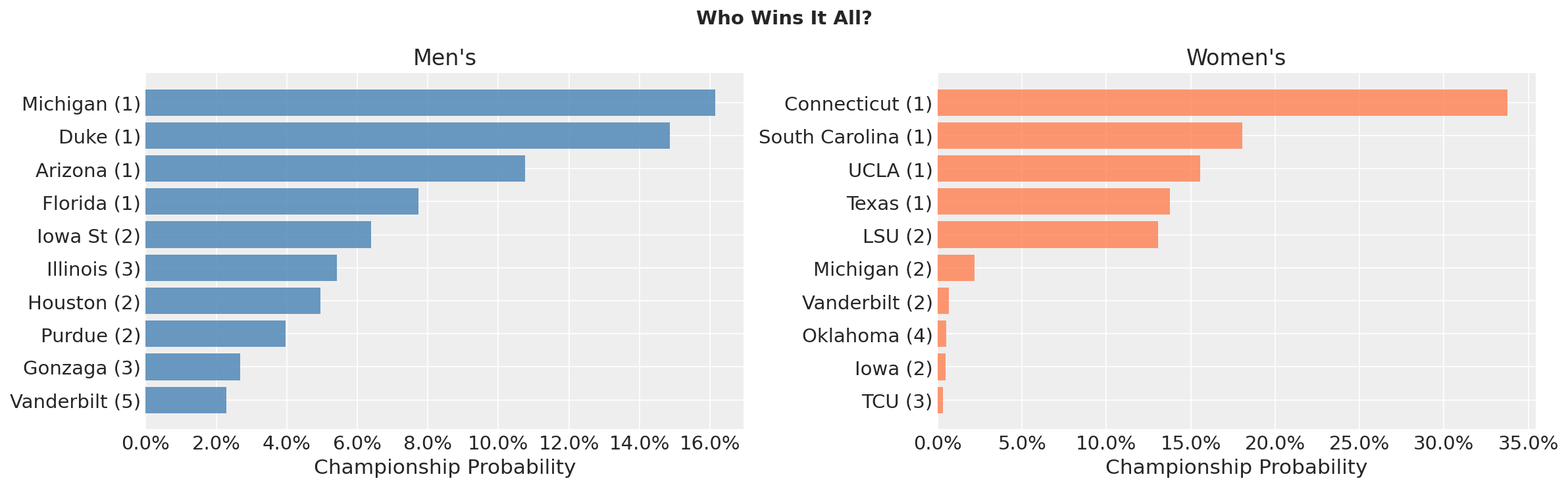
Team	Seed	P(Champion)
Connecticut	1	33.8%
South Carolina	1	18.1%
UCLA	1	15.6%
Texas	1	13.8%
LSU	2	13.1%

UConn’s 34-0 record translates to a posterior strength distribution that clearly leads the pack, they are elite on both offense and defense.

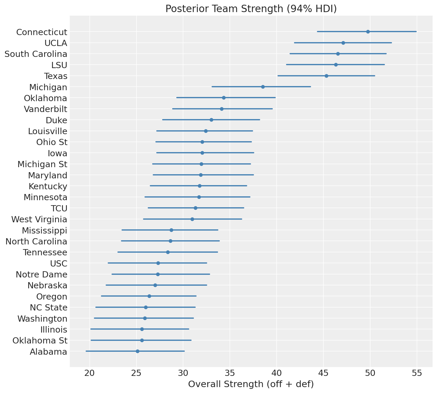
The structural difference between the men’s and women’s fields is stark. The men’s top 30 is a smooth gradient where each team’s HDI overlaps with the teams around it. The women’s field has a clear break: five teams in one tier, Texas sort of in-between, then below that, the rest of the tournament field packs into a narrow band.

Talent in women’s college basketball is less equitably distributed. The top programs separate themselves from the field by a wider margin than their men’s counterparts, and the model sees it directly in the regular season results. For one, the correlation between offense and defense is much stronger in the women’s tournament.

We can quantify the concentration with a Gini coefficient over championship probabilities (0 means every team has equal odds, 1 means a single team wins every simulation). The women’s field is substantially more top-heavy: a Gini of 0.93 compared to 0.79 for the men’s. Put differently, only 29 women’s teams won the title in any of 10,000 simulations, compared to 46 on the men’s side.

Women’s Advancement Probabilities

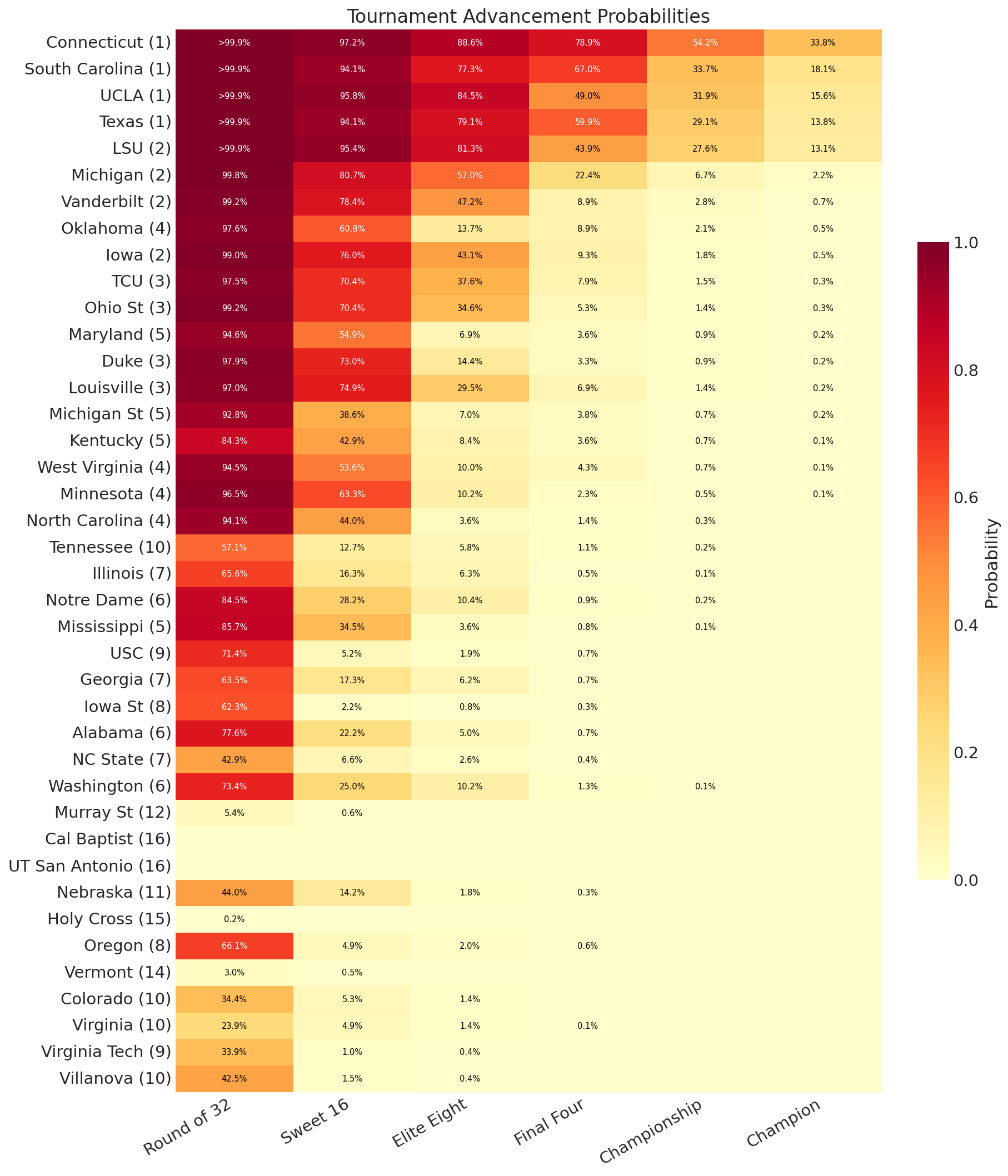
The advancement heatmap makes the concentration visible. The women’s top seeds are a sea of deep red through the Sweet 16 and beyond, while probability drops off far more sharply for everyone else.

Home Court Advantage: This Time it Actually Matters

The women’s model estimates \(\alpha\) at 1.37 ± 0.10, almost identical to the men’s 1.44. The posteriors overlap almost entirely, suggesting that home court is roughly the same phenomenon across genders (a margin effect of about 2.7-2.9 points).

It is worth noting that this affects predictions differently than in the men’s tournament. In the men’s tournament, every game is neutral-site, so home court zeros out entirely. In the women’s tournament, the top 16 seeds host rounds 1 and 2 on their home courts. That ~2.8-point margin advantage compounds on top of the strength differential that already favors higher seeds, making the early rounds even more lopsided.

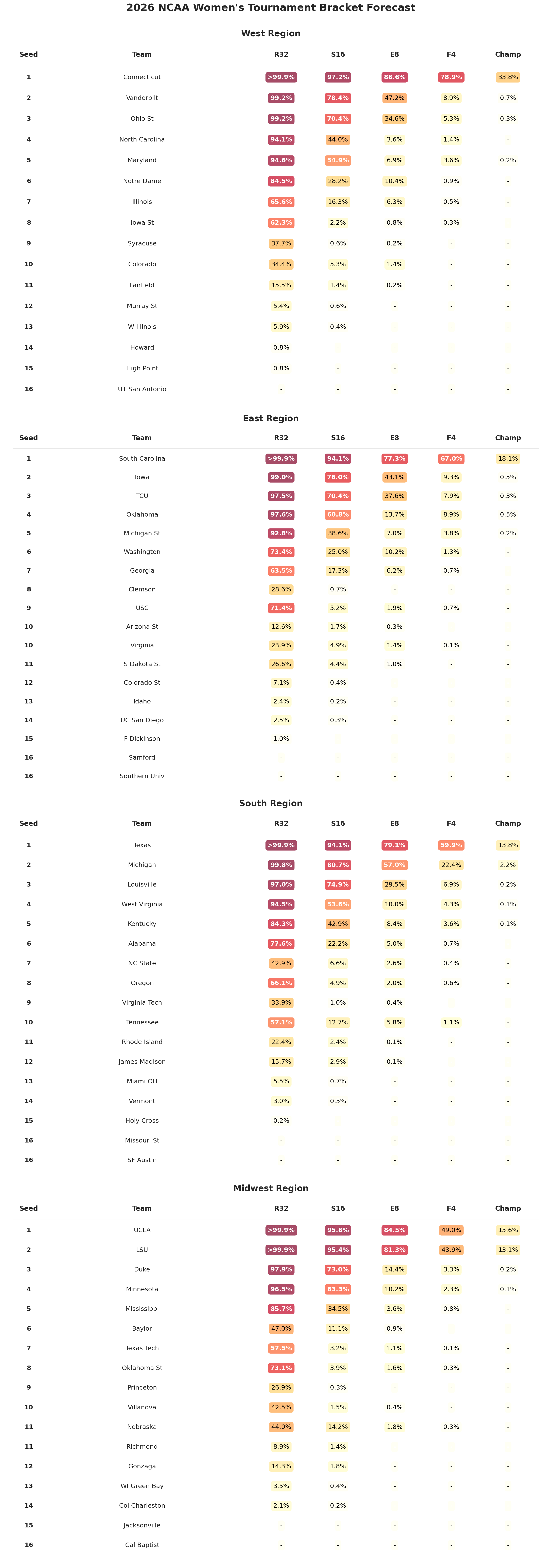
The Brackets

Based on the most likely outcome at each matchup:

Men’s

Final Four: Duke, Florida, Michigan, Arizona

Championship Game: Michigan vs. Duke

Champion: Michigan (16.2%, meaning we’re 83.8% sure this is wrong)

Women’s

Final Four: UConn, South Carolina, UCLA, Texas

Championship Game: UConn vs. South Carolina

Champion: UConn (33.8%, meaning we’re 66.2% sure this is wrong)

The contrast captures the structural difference between the two fields. The men’s champion is nearly a coin-flip among three or four teams. The women’s champion is the clearest favorite the model produces, but 33.8% still means there’s a 66.2% chance that UConn loses. Single-elimination tournaments are designed to produce uncertainty, and even a dominant team can only be so dominant across six consecutive games.

Following Along

I’ve put together an interactive dashboard that will update daily as the tournament progresses, so you can watch the model’s predictions shift as games are played and teams are eliminated. It is worth noting that these predictions run the statistical model live every morning, meaning there may be relatively small differences between predictions here and the dashboard, since I do not fix the random seed.

I also submitted these predictions to the Kaggle March ML Mania 2026 competition to see how they stack up against other approaches. By no means do I expect this to win, since it’s more a pedagogy-first exercise and more feature-dense approaches will likely perform better. That being said, it will be fun for a performance comparison.

Code

All code for this analysis is available on GitHub.